Understanding GC pauses in JVM, HotSpot's CMS collector.

Concurrent Mark Sweep (CMS) is one of HotSpot JVM low pause garbage collectors. CMS can do most of its work for reclaiming memory concurrently with application (without stopping it). But still it requires few stop-the-world pauses to make its work. This article will explain nature of these pauses and how to minimize them.

Basics of concurrent mark sweep

HotSpot’s CMS is a generational collector, it means that heap is separated into young and old (tenured) space and these spaces are collected independently. For young space collection usual HotSpot’s copy collector is use (see previous article about HotSpot’s young space collector).  To enable of using CMS collector you have to specify ‑XX: +UseConcMarkSweepGC in JVM’s command line.

Concurrent Mark Sweep is used only to collect old space. CMS collection cycle has following phases:

• Initial mark – this is stop-the-world phase while CMS is collecting root references.
•  Concurrent mark – this phase is done concurrently with application, garbage collector traverses though object graph in old space marking live objects.
• Concurrent pre clean – this is another concurrent phase, basically it is another mark phase which will try to account references changed during previous mark phase. Main reason for this phase is reduce time of stop-the-world remark phase.
• Remark – once concurrent mark is finished, garbage collector need one more stop-the-world pause to account references which have been changed during concurrent mark phase.
• Concurrent sweep – garbage collector will scan through whole old space and reclaim space occupied by unreachable objects.
• Concurrent reset – after CMS cycle is finished, some structures have to be reset before next cycle can start.

Unlike most other garbage collectors, CMS does not do compaction of heap space. Instead of moving objects to make unoccupied space continuous, CMS keeps lists of all fragments of free memory. This way CMS is avoiding cost associated with relocating of live objects (and relocating of objects is expensive operation which require stop-the-world pause), but as down size of this heap space is prone to fragmentation. To minimize risk of fragmentation CMS is doing statistical analysis of object’s sizes and have separate free lists for objects of different sizes.

Length of CMS pauses

CMS itself has only two pauses, but your application will also experience pauses of young space collector which is working in conjunction with CMS. See previous article about pauses of young space collector.

Initial mark

During   initial mark CMS should collect all root references to start marking of old space. This includes:

• References from thread stacks,
• References from young space.

References from stacks are usually collected very quickly (less than 1ms), but time to collect references from young space depends on size of objects in young space. Normally initial mark starts right after young space collection, so Eden space is empty and only live objects are in one of survivor space. Survivor space is usually small and initial mark after young space collection often takes less than millisecond. But if initial mark is started when Eden is full it may take quite long (usually longer than young space collection itself).

Once CMS collection is triggered, JVM may wait some time for young collection to happen before it will start initial marking. JVM configuration option –XX:CMSWaitDuration=<t> can be used to set how long CMS will wait for young space collection before start of initial marking. If you want to avoid long initial marking pauses, you should configure this time to be longer than typical period of young collections in your application.

Remark

Most of marking is done in parallel with application, but it may not be accurate because application may modify object graph during marking. When concurrent marking is finished; garbage collector should stop application and repeat marking to be sure that all reachable objects marked as alive. But collector doesn’t have to traverse through whole object graph; it should traverse only reference modified since start of marking (actually since start pre clean phase). Card table (see card marking write barrier) is used to identify modified portions of memory in old space, but thread stacks and young space should be scanned once again.

 Usually most time of remark phase is spent of scanning young space. This time will be much shorter if we collect garbage in young space before starting of remark. We can instruct JVM to always force young space collection before CMS remark. Use JVM parameter –XX:+CMSScavengeBeforeRemark to enable this option.

Even is young space is empty, remark phase still have to scan through modified references in old space, this usually takes time close to normal young collection pause (due scanning of old space done during young collection is similar to scanning required for remark).

When CMS collection starts?

Unlike stop-the-world old space collectors, CMS collection cycle should start before old space become full. CMS collection is triggered when amount of free memory in old space falls below certain threshold (this threshold can be chosen by JVM based of runtime statistics or set via parameters) and actual start of CMS collection cycle may be delayed until next young collection.

Normally objects are allocated in old space only during young space collection (which may promote some objects to old space). So CMS cycle usually starts right after young space collection, which is good because init mark pause will be very small.

But in certain cases object may be allocated directly in old space and CMS cycle could start while Eden has lots of objects. In this case initial mark can be 10-100 times slower which is bad. Usually this is happening due to allocation of very large objects (few megabyte arrays).  To avoid these long pauses you should configure reasonable –XX:CMSWaitDuration.

Configuring fixed threshold for CMS start

You can set fixed threshold for olds space occupation for triggering CMS cycle by using JVM options ‑XX:+UseCMSInitiatingOccupancyOnly ‑XX:CMSInitiatingOccupancyFraction=70 (this will force CMS cycle to start when more than 70% of old space is used).

Explicitly invoking CMS cycle

You can also configure JVM to start CMS cycle by invocation of System.gc() by ‑XX:+ExplicitGCInvokesConcurrent command line option.

Full GC with CMS

If CMS cannot free enough in old space, JVM may fallback to compacting collector. Compacting collector will force stop-the-world pause so it can be considered emergency case. Normally you would like to avoid full GC and long stop-the-world pause associated with it. Full GC may happen either if CMS is not fast enough for dealing with garbage (or collection cycle has been started too late) or due to fragmentation of old space (there is no large enough continuous space for object to be allocated). Also it is possible that you just didn’t give JVM enough memory and after full GC it will through OutOfMemoryExpection anyway.

Permanent generation collection

One of reasons why CMS may end up in full GC is garbage in permanent space. By default CMS does not reclaim unused space in permanent space. If your application is using multiple class loaders and/or reflection you may need to enable collecting of garbage in permanent space. JVM option ‑XX:+CMSClassUnloadingEnabled will allow CMS collector to clean permanent space. Remember that objects in permanent space may have references to normal old space thus even if permanent space is not full itself, references from perm to old space may keep some dead objects unreachable for CMS if class unloading is not enabled.

Utilizing multiple cores

CMS has multiple phases. Some of them are concurrent; others are stop-the-world pauses but may be executed in parallel to compressed application freeze time.

‑XX:+CMSConcurrentMTEnabled – allows CMS to use multiple cores for concurrent phase.

‑XX:ConcGCThreads=<n> – specifies number of thread for concurrent phases.

‑XX:ParallelGCThreads=<n> – specifies number of thread for parallel work during stop-the-world pauses (by default it equals to number of physical cores).

‑XX:+UseParNewGC – instructs JVM to use parallel collector for young space collections in conjunction with CMS.

See also

HotSpot JVM garbage collection options cheat sheet 
Java GC, HotSpot's CMS and heap fragmentation
Other articles about garbage collection in this blog

Understanding GC pauses in JVM, HotSpot's minor GC.

Stop the world pauses of JVM due to work of garbage collector are known foes of java based application. HotSpot JVM has a set of very advanced and tunable garbage collectors, but to find optimal configuration it is very important to understand an exact mechanics garbage collection algorithms. This article one of series explaining how exactly GC spends our precious CPU cycle during stop-the-world pauses. An algorithm for young space garbage collection in HotSpot is explained in this issue.

Structure of heap

Most of modern GCs are generational. That means java heap memory is separated into few spaces. Spaces are usually distinguished by “age” of objects. Objects are allocated in young space, then, if they survive long enough, eventually promoted to old (tenured) space. That approach rely on hypothesis that most object “die young”, i.e. majority of objects are becoming garbage shortly after being allocated. All HotSpot garbage collectors are separating memory into 5 spaces (though for G1 collector spaces may not be continuous).

• Eden are space there objects are allocated,
• Survivor spaces are used to receive object during young (or minor GC),
• Tenured space is for long lived objects,
• Permanent space is for JVM own objects (like classes and JITed code), it is behaves very like tenured space so we will ignore it for rest of article.

Eden and 2 survivor spaces together are called young space.

HotSpot GC algorithms overview

HotSpot JVM is implementing few algorithms for GC which are combined in few possible GC profiles.

• Serial generational collector (-XX:+UseSerialGC).
• Parallel for young space, serial for old space generational collector (-XX:+UseParallelGC).
• Parallel young and old space generational collector (-XX:+UseParallelOldGC).
• Concurrent mark sweep with serial young space collector (-XX:+UseConcMarkSweepGC
  –XX:-UseParNewGC).
• Concurrent mark sweep with parallel young space collector (-XX:+UseConcMarkSweepGC –XX:+UseParNewGC).
• G1 garbage collector (-XX:+UseG1GC).

All profiles except G1 are using almost same young space collection algorithms (with serial vs parallel variations).

Write barrier

Key point of generational GC is what it does need to collect entire heap each time, but just portion of it (e.g. young space). But to achieve this JVM have to implement special machinery called “write barrier”. There 2 types of write barriers implemented in HotSpot: dirty cards and snapshot-at-the-beginning (SATB). SATB write barrier is used in G1 algorithms (which is not covered in this article). All other algorithms are using dirty cards.

Dirty cards write-barrier (card marking)

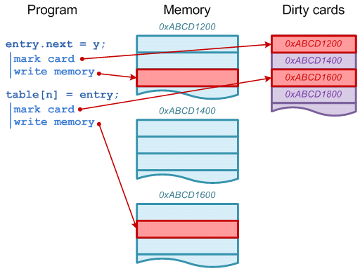
Principle of dirty card write-barrier is very simple. Each time when program modifies reference in memory, it should mark modified memory page as dirty. There is a special card table in JVM and each 512 byte page of memory has associated byte in card table.

Young space collection algorithm

Almost all new objects (there are few exception when new object can be allocated directly in old space) are allocated in Eden space. To be more effective HotSpot is using thread local allocation blocks (TLAB) for allocation of new objects, but TLAB themselves are allocated in Eden. Once Eden becomes full minor GC is triggered. Goal of minor GC is to clear fresh garbage in Eden space. Copy-collection algorithm is used (live objects are copied to another space, and then whole space is marked as free memory). But before start collecting live objects, JVM should find all root references. Root references for minor GC are references from stack and all references from old space.

Normally collection of all reference from old space will require scanning through all objects in old space. That is why we need write-barrier. All objects in young space have been created (or relocated) since last reset of write-barrier, so non-dirty pages cannot have references into young space. This means we can scan only object in dirty pages.

Once initial reference set is collected, dirty cards are reset and JVM starts coping of live objects from Eden and one of survivor spaces into other survivor space. JVM only need to spend time on live objects. Relocating of object also requires updating of references pointing to it.

While JVM is updating references to relocated object, memory pages get marked again, so we can be sure what on next young GC only dirty pages has references to young space.

Finally we have Eden and one survivor space clean (and ready for allocation) and one survivor space filled with objects.

Object promotion

If object is not cleared during young GC it will be eventually copied (promoted) to old space. Promotion occurs in following situations:

• -XX:+AlwaysTenure  makes JVM to promote objects directly to old space instead of survivor  space (survivor spaces are not used in this case).
• once survivor space is full, all remaining live object are relocated directly to old space.
• If object has survived certain number of young space collections, it will be promoted to old space (required number of collections can be adjusted using –XX:MaxTenuringThreshold option and –XX:TargetSurvivorRatio JVM options).

Allocation of new objects in old space

It would be beneficial if we could possibly allocate long lived objects directly in old space. Unfortunately there is no way to instruct JVM to do this for particular object. But there are few cases when object can be allocated directly in old space.

• Option -XX:PretenureSizeThreshold=<n> instructs JVM what all objects larger  than <n> bytes should be allocated directly in old space (though if object size fits TLAB, JVM will allocate it in TLAB and thus young space, so you should also limit TLAB size).
• If object is larger than size of Eden space it also will be allocated in old space.

Unlike application objects, system objects are always allocated by JVM directly in permanent space.

Parallel execution

Most of task during young space collection can be done in parallel. If there are several CPUs available, JVM can utilize them to compress duration of stop-the-world pause during collection. Number of threads can be configured in HotSpot JVM by –XX:ParallelGCTreads= parameter. By default JVM will choose number of thread by number of available CPU. As expected, serial version of collector will ignore this parameter because it can use only one CPU. Using parallel collection reduces time of stop-the-world pause by factor close to number of physical cores.

Time of young GC

Young space collection happens during stop-the-world pause (all non-GC-related threads in JVM are suspended). Wall clock time of stop-the-world pause is very important factor for applications (especially applications requiring fast response time). Parallel execution affects wall clock time of pause but not work effort to be done.

Let’s summarize components of young GC pause. Total pause time can be written as:

T_young = T_{stack_scan} + T_card__scan + T_old__scan+ T_copy ; there T_young is total time of young GC pause, T_{stack_scan} is time to scan root in stacks, T_card__scan is time to scan card table to find dirty pages, T_old__scan  is time to scan roots in old space and T_copy is time to copy live objects (1).

Thread stack are usually very small, so major factors affecting time of young GC is T_card__scan , T_old__scan and T_copy.

Another important parameter is frequency of young GC. Period between young collections is mainly determined by application allocation rate (bytes per second) and size of Eden space.

P_young = S_eden / R_alloc ; there P_young  is period between young GC, S_eden is size of Eden and R_alloc is rate of memory allocations (bytes per second) (2).

T_{stack_scan} – can be considered application specific constant.

T_{card_scan} – is proportional to size of old space. Literally, JVM have to check single byte of table for each 512 bytes of heap (e.g. 8G of heap -> 16m to scan).

T_old__scan  – is proportional to number of dirty cards in old space at the moment of young GC. If we assume that references to young space are distributed randomly in old space, then we can provide following formula for time of old space scanning.

; there S_old is size of old space and D, k_card and n_card are coefficients specific for application (3).

T_copy – is proportional to number of live objects in heap. We can approximate it by formula:

There k_copy is effort to copy object, R_{long_live} is rate of allocation of long lived objects,  

(k_survive usually very small), and k_tenure is a coefficient to approximate aging of object in young space before tenuring (k_tenure ≥ 1) (4).

Now we can analyze how various JVM options may affect time and frequency of young GC.

Size of old space.

Size of old space is affecting T_{card_scan} and T_{old_scan} part of young GC pause time according to formulas above. So we as we are increasing size of old space (read total heap size) time of young GC pauses will grow and it cannot be helped. After certain size of heap (usually 4-8 Gb) time of young collection is dominated by T_{card_scan} (technically T_copy can be even greater than T_{card_scan} , but it usually can be controlled by tuning of other GC options).

HotSpot JVM options:

-Xmx=<n> -Xms=<n>

Size of Eden space 

Period between young GC is proportional to size of Eden. T_copy is also proportional to size of eden but in practice k_survive can be so small that for some applications we can forget about Tcopy. Unfortunately time between young GC will also affect coefficient D in equation (4). Though dependency between D and P_young is very application specific, increasing P_young will increase D and as a consequence T_{scan_old}.

HotSpot JVM options:

-XX:NewSize=<n> -XX:MaxNewSize=<n>

Size of survivor space. 

Size of survivor space puts hard limit of how much objects can stay in young space between collections. Changing size of survivor space may affect k_tenure (or mat not, e.g. if k_tenure is already 1).

HotSpot JVM options:

-XX:SurviorRatio=<n>

Max tenuring threshold and target survivor ratio 

These two JVM options also allow artificially adjust k_tenure.

HotSpot JVM options:

-XX:TargetSurviorRatio=<n>
‑XX:MaxTenuringThreshold=<n>
-XX:+AlwaysTenure
-XX:+NeverTenure

Pretenuring threshold 

For certain applications using pretenuring threshold could reduce k_survive due to allocation of long lived object directly in old space.

HotSpot JVM options:

-XX:PretenureThreshold=<n>

See also

Other articles about garbage collection in this blog

Indexes: RDBMS vs Coherence vs Lucene

Techincal article comparing popular indexing algorithms between RDBMS, data grid (Oracle Coherence) and full text search engine (Lucene).

Most people are familiar with concept of “index” in SQL database. But indexes are widely used far beyond relational databases. There are even dedicated products, like search engines, which are specializing in indexing of data stored elsewhere. This article will give a high level comparison of capabilities and performance aspects of typical indexes in three different types of technologies: SQL database, in-memory-data-grid (Oracle Coherence) and full text search engine (Apache Lucene).

Full text of article is available at GridDynamics blog - http://blog.griddynamics.com/2011/04/indexes-rdbms-vs-coherence-vs-lucene.html

Coherence, magic trick with cache index

A technical article related to Oracle Coherence.

Oracle Coherence has ability to query data in cache not only by key, but by values (or their attributes). Of course queering by secondary attributes is not as efficient as by primary key, but still can be very useful. Oracle Coherence also supports indexes which improve performance of value based queries significantly.
But some times index may not behave exactly as you expect.

Full text of article is available at GridDynamics blog - http://blog.griddynamics.com/2010/10/coherence-magic-trick-with-cache-index.html

Coherence, ReflectionPofSerializer now supports POF extractor

A technical article related to Oracle Coherence.

A year ago I have implemented and open sourced ReflectionPofSerializer. This class has saved me from implementing thousands of lines of boring serialization code for various Filters, EntryProcessors, Aggregators , Invocables and other mobile objects in Coherence.

Recently I was asked about POF extrator support in ReflectionPofSerializer. My answer was no, it doesn't support extraction from POF directly. But it turns out what ReflectionPofSerializer can be easily extended to support it. A bit of coding and woala, let me introduce ReflectionPofExtrator.

Full text of article is available at GridDynamics blog - http://blog.griddynamics.com/2010/07/coherence-reflectionpofserializer-now.html

Coherence. Read through and operation bundling.

A technical article about Oracle Coherence data grid.

If you are using read-write-backing-map, you should know what CacheLoader interface has methods load(...) and loadAll(…) for bulk loading. And if your cache loader is loading data from DB, your implementation of loadAll(…) is probably designed to load all objects via single DB query (cause it is usually order of magnitude more efficient than issue DB query per requested key). Lets assume your read through cache is working just fine, and at some point you decided to implement cache preloading – a popular pattern. To implement preloading you have found some way to collect keys (e.g. via query to DB) and wanted to use getAll(…) call to load data into cache. Everything looks ok, unit tests have passed, but on real data it takes forever to preload cache! Let’s investigate this …

Full text of article is available at GridDynamics blog - http://blog.griddynamics.com/2010/06/coherence-read-through-and-operation.html

4 levels of replication technologies

Esse about state of art in replication technologies.

Replication is widely used to achieve various goals in information systems, such as better performance, fault tolerance, backup, etc. Four classes of replication technologies are available. Your decision about which technology to use will depend on the logical presentation of the data you are trying to replicate.

Full text of article is available at GridDynamics blog - http://blog.griddynamics.com/2010/02/4-levels-of-replication-technologies.html

Data storages and read vs write controversy

While working with various high-loaded systems recently, I noticed a paradoxical contradiction in the data models. Let me explain through the following comparisons. First let's think about normalized vs. denormalized data models.

	Normalized	Denormalized
Read	Bad - Queries become complex - Joins and nested selects are slow	Good - Fast queries - No joins - Queries are mostly single index lookup (assuming schema is tailored for application need)
Write	Good - Consistency is easier to keep - No self contraction by schema - Less rows to update	Bad - Potential inconsistency in data - More rows to update (data may be duplicated in several places) - Complex update procedures

Let's continue with the next comparison -- single vs. multiple copies of data.

	Single copy	Multiple copies
Read	Bad - Single copy is bottleneck	Good - Operations can be balanced between copies
Write	Good - No need to keep copies in sync - Single place to update	Bad - Update should performed at every copy - Synchronization and consistency issues - Transactional updates become distributed transactions

In general, the patterns are simple. If we think of our data as a set of facts, we anticipate each fact will become several data records (either though database replicas or denormalization of the model). For write access, dealing with each fact as a single record is much more efficient. The impact of this difference between what is and what should be can mitigated by using the optimal storage technology for a given application.

The picture above is very simple (or even simplistic) but it provides some insight for selecting the proper data storage for your applications (or even specific parts of your application). If you have any comments about this, please reply to this post.

Key/value and document-oriented storages

These are data-storage techniques that don't support joins and they usually break the 1^st normal form. Due to limited query support, the schema is often prepared in such a way that application queries become simple index lookups. This can be a very effective approach, but the flip side of this is usually a duplication of the entity's attributes across several tables (or their analogs). This makes updating of data more expensive. These types of storages also tending to use asynchronous disk operations which is further undermine their value as system of record storage. Lack of ACID properties is also of no help.

Search indexes

Search indexes such as Lucene and Sphynx provide excellent query performance. They are using data structures designed for information retrieval at cost of expensive updates. Search engines also require denormalized data model, further complicating writes.

RDBMS

Relational databases have a strong reliance on normalization of the data model. It is extremely difficult for an RDBMS to be effective for both read and write operations. While an RDBMS will never be as fast or as simple as a key/value hash table because the write operations will always be quite expensive (due to indexes and consistency checks), they can be a good middle ground between key/value hash tables and MQ-based storage.

MQ

It may be surprising to some people that I have included message queues in the same discussion with databases. But persistent queues or publish/subscribe systems with quarantined delivery are similar to databases. Submitting a message is like a write operation and receiving a message is like a read. The important thing about MQs is that they can be very efficient for write operations. Read operations in MQ environments are very limited, but experience has shown that "write-only" data storage can fill an important niche.

Convergence of paradigms

In the early days of relational databases, many people were skeptical about their future. The main argument against them was performance. But RDBMS technology has survived. Vendors have made the indexes faster and the query optimizers smarter. Overall, the performance and reliability have improved significantly. While maintaining a strong position in their niche, they have slowly assimilated key features of competing technologies to expand their appeal.

Materialized views are actually a smart way to get the benefits of denormalized data while keeping the schema normalized when it comes to updating. Message queues are also becoming a part of RDBMS offerings (e.g., Oracle RDBMS has queues at its core and PostgreSQL has production-ready built-in queues used by Skype).

We are living in an interesting time. Networking has led to the exponential growth in the amount of data created by, and use for, applications. Data-storage technologies have to adapt and evolve quickly, and it's fascinating to watch this evolution. Good luck with your data storage!

Java tricks, reducing memory consumption

In this blog post, I want to discuss optimization of java memory usage. The Sun JDK has two simple-but-powerful tools for memory profiling – jmap and jhat.

jmap has two important capabilities for memory profiling. It can:

• create a heap dump file for any live java process
• show a heap distribution histogram

Neither of these capabilities requires any special parameters for the Java virtual machine (JVM). Below is a heap distribution histogram produced by jmap.

>jmap -histo:live 16608
num     #instances         #bytes  class name
----------------------------------------------
   1:        260317       25199232  [C
   2:        166085       24205896 
   3:        265765       13336072 
   4:        166085       13304504 
   5:         15645        9921728 
   6:        295513        7092312  java.lang.String
   7:         27721        7048392  [I
   8:         15645        7032592 
   9:         12920        5839232 
  10:         20621        5702816  [B
  11:         27440        3493744  [Ljava.util.HashMap$Entry;
  12:        140640        3375360  java.util.HashMap$Entry
  13:        102400        3276800  org.jboss.netty.util.internal.ConcurrentIdentityHashMap$Segment
  14:        102400        3276800  [Lorg.jboss.netty.util.internal.ConcurrentIdentityHashMap$HashEntry;
  15:         51198        2880304  [Ljava.lang.Object;
  16:        106925        2566200  java.util.concurrent.locks.ReentrantLock$NonfairSync
  17:         22668        1693408  [S
  18:         16749        1607904  java.lang.Class
  19:         23731        1086064  [[I
  20:         30176        1060240  [Ljava.lang.String;
  21:         25600        1024000  org.jboss.netty.util.internal.ConcurrentIdentityHashMap
  22:         25600        1024000  org.jboss.netty.util.internal.ConcurrentIdentityHashMap$KeyIterator
  23:         29038         929216  java.util.LinkedHashMap$Entry
  24:         22857         914280  java.util.HashMap
  25:         13255         848320  org.eclipse.core.internal.resources.ResourceInfo
  26:         25600         819200  [Lorg.jboss.netty.util.internal.ConcurrentIdentityHashMap$Segment;
  27:         17506         805264  [[C
  28:         27531         660744  java.util.ArrayList
...
Total       2587755      166479680

For each class we can see the class name, the number of instances of the class in the heap, and the number of bytes used in the heap by all instances of the class. The table is sorted by consumed heap space. Although it is very simple, it is extremely useful. This information is enough to diagnose 60% of heap capacity problems.

[ symbol before class name means that it is array of objects, arrays of primitive types look like
[B - for byte[]
[C - for char[]
[I - for int[]

If a heap distribution histogram is too high-level, you can try jhat. jhat can read and explore a heap dump. It has a web interface and you can click though your dumped object graph. Of course, clicking through a few million objects is not fun. Fortunately, jhat supports query language. Let's give it a try.

>jmap -dump:file=eclipse.heap 16608
Dumping heap to C:\Program Files (x86)\Java\jdk1.6.0_11\bin\eclipse.heap ...
Heap dump file created

>jhat -J-Xmx1G eclipse.heap
Reading from eclipse.heap...
Dump file created Wed Oct 14 08:41:07 MSD 2009
Snapshot read, resolving...
Resolving 2300585 objects...
Chasing references, expect 460 dots.............................................
................................................................................
................................................................................
.......................................
Eliminating duplicate references................................................
................................................................................
................................................................................
....................................
Snapshot resolved.
Started HTTP server on port 7000
Server is ready.

Now open http://localhost:7000 and you can see a summary of all classes. You can use standard queries via links or go straight to the “Execute Object Query Language (OQL) query” link at the bottom and type your own query. Query language is quite awkward (it is based on the java script engine) and may not work well for large numbers of objects, but it is a very powerful tool.

Enterprise applications are 80% strings and maps

Let’s look at the jmap histogram again. In the top row, we can see "[C" class consuming most of the heap space. Actually, these char arrays are part of String objects, and we can see that String instances are also consuming considerable space. From my experience, 60-80% of heaps in an enterprise application are consumed by strings and hash maps.

Strings

Let's look how the JVM is storing strings. String objects are semantically immutable. Each instance has four fields (all except hash are marked final):
  •  Reference to char array
  •  Integer offset
  •  Integer count of character
  •  Integer string hash (lazily evaluated, and once evaluated never changes)

How much memory does one String instance consume?

Here and below are size calculations for the Sun JVM (32bit). This should be similar for other vendors.
Object header (8 bytes) + 3 refs (12 bytes) + int (4 bytes) = 24 bytes. But the String instance is only a header. Actual text is stored in char array (2 bytes each character + 12 bytes array header).

String instances can share char arrays with each other. When you call substring(…) on a String instance, no new char array allocation happens. Instead, a new String referencing subrange of existing char arrays is created. Sometimes this can become a problem. Imagine you are loading a text file (e.g., CSV). First you are loading the entre line as string, then you seek the position of the field and call substring(…). Now your small field value string object has a reference to an entry line of text. Sometime later, a string header for the text line object is collected, but characters are still in memory because they are referenced via other string object.

In the illustration above, useful data is marked by yellow. We can see that some characters cannot be accessed any more, but still occupy space in the heap. How can you avoid such problems?
If you are creating a String object with a constructor, a new char array is always allocated. To copy content of a substring you can use the following construct (it looks a bit strange, but it works):
new String(a.substring(…))

String.intern() – think twice

String class has a method intern() that can guarantee the following:
a.equals(b)  => a.intern() == b.intern()
There is a table inside of the JVM used to store normal forms of strings. If some text is found in a table then value from a table will be returned from intern(), else the string will be added to table. So a reference returned by intern() is always an object from JVM intern table.

String intern table keep weak references to its objects, so unused strings can be collected as garbage when no other references exist except from intern table itself. It looks like a great idea to use intern(), and eliminate all duplicated strings in an application. Many have tried … and many have regretted such decision. I cannot say this is true for every JVM vendor, but if you are using Sun’s JVM, you should never do this.
Why?

• JVM string intern tables are stored in PermGen – a separate region of the heap (not included in ‑Xmx size) used for the JVM’s internal needs. Garbage collection in this area is expensive and size is limited (though configurable).
• You would have to insert a new string into the table which has O(n) complexity, where n is table size.

String intern tables in JVMs work perfectly for the JVM’s needs (new entries are added only while loading new classes so insertion time is not a big issue) and it is very compact. But it is completely unsuitable for storing millions of application strings. It just was not designed for such a use case.

Removing of duplicates

The JVM’s string intern table is not an option but the idea of eliminating string duplicates is very attractive. What can we do?

public
class InternTable {

 private
   final Map table = new HashMap();

 public X intern(X val) {
  X in = table.get(val);
  if (in == null) {
  table.put(val, val);
  in = val;
  }
  return in;
  }
}

Above is a simple snippet of a custom intern table. It can be used for strings or any other immutable objects. Looks good, but it has a problem. Such an implementation will prevent objects from being collected by GC. What can we do?

We need to use weak references. There are WeakHashMap classes in the JDK. It is a hash table that uses weak references for keys. Let's try to use it.

public
class InterTable {

private
final Map table = new WeakHashMap();

public X intern(X val) {
  WeakReference ref = table.get(val);
  X in = ref == null ? null : ref.get();
  if (in == null) {
    table.put(val, new WeakReference(val));
    in = val;
  }
  return in;
 }
}

Did you notice we also need a weak reference for the wrap value? This will work, but what is the cost?
  •  Reference from hash table – 1 ref * ratio of unused slots (~6 bytes)
  •  WeakHashMap$Entry object – 40 bytes
  •  value WeakReference – 24 bytes

The cost per entry in the table is about 70 bytes. That’s expensive. Can we reduce it?

Right now we have to have two weak references per entry. If we rewrite WeakHashMap to return an entry from the get(...) method (instead of the value), we can drop the second weak reference and save 24 bytes. But the cost of such an intern table is still high. You should analyze/experiment with your data to see if such a trick will bring greater benefits in your case.

UTF8 strings

Java strings are UTF and encoded using UTF16 in memory. If they are to be converted to UTF8, the actual text is likely to consume half the memory. But using UTF8 will break compatibility with the String class. You have to create your own class and convert it to standard String for a majority of operations. This will increase CPU usage, but in some edge cases this approach can be useful for overcoming heap size limitations (e.g., storing large text indexes in memory).

Maps and sets

Old good HashMap

Good old java.util.HashMap is used everywhere. Standard implementation in JDKs is to use the open hash table data structure.

References to key and value are stored in the Entry object (which also keeps the hash for the key for faster access). If several keys are mapped to same hash slot, they are stored as a list of interlinked entries. The size of each entry structure: object header + 3 references + int = 24 bytes. java.util.HashSet is using java.util.HashMap under the hood so your overhead will be the same.
Can we store map/set in more compact form?
Sure.

Sorted array map

If the keys are comparable, we can store the map or set as sorted arrays of interleaved key/value pairs (array of keys in the case of a set). Binary search can be used for fast lookups in an array, but insertion and deletion of entries will have to shift elements. Due to the high cost of updates in such a structure, it will be effective only for smaller collection sizes, and for operation patterns that are mostly read. Fortunately, this is usually what we have – map/set of a few dozen objects that are read more often than modified.

Closed hash table

If we have a collection of a larger size, we should use a hashtable. Can we make the hashtable more compact? Again, the answer is yes. There are data structures called closed hashtables that do not require entry objects.

In closed hashtables, references from the hashtable point directly to an object (key). What if we want to put in a reference to a key but the hash slot is occupied already? In such a case, we should find another slot (e.g., next one). How do you lookup a key? Search through all adjacent slots until key or null reference is found. As you can see from algorithm, it is very important to have enough empty slots in your table. Density of closed hash tables should be kept below 0.5 to avoid performance degradation.

Maps structures summary

Open hash map/set Cost per entry: 1 ref * 1.33 (for 0.75 density) Entry object Total: ~30 bytes + Better handling hash collisions. + Fast access to hash code.

Closed hash map/set Cost per entry (map): 2 ref * 2 (for 0.5 density) Total: 16 bytes Cost per entry (set): 1 ref * 2 (for 0.5 density) Total: 8 bytes - Generally slower than open version.

Sorted array map/ser Cost per entry (map): 2 ref Total: 8 bytes Cost per entry (set): 1 ref Total: 4 bytes - For small collection only. - Expensive update/delete.

The JDK is using an open hashtable structure because in general case it is a better structure. But when you are desperate to save memory, the other two options are worth considering.

Conclusion

Optimization is an art. There are no magical data structures capable of solving every problem. As you can see, you have to fight for every byte. Memory optimization is a complex process. Remember that you should design your data so each object can be referenced from different collections (instead of having to copy data). It is usually better to use semantically immutable objects because you can easily share them instead of copying them. And from my experience, in a well-designed application, optimization and tuning can reduce memory usage by 30-50%. If you have a very large amount of data, you have to be ready to handle it.