Understanding GC pauses in JVM, HotSpot's minor GC.

Stop the world pauses of JVM due to work of garbage collector are known foes of java based application. HotSpot JVM has a set of very advanced and tunable garbage collectors, but to find optimal configuration it is very important to understand an exact mechanics garbage collection algorithms. This article one of series explaining how exactly GC spends our precious CPU cycle during stop-the-world pauses. An algorithm for young space garbage collection in HotSpot is explained in this issue.

Structure of heap

Most of modern GCs are generational. That means java heap memory is separated into few spaces. Spaces are usually distinguished by “age” of objects. Objects are allocated in young space, then, if they survive long enough, eventually promoted to old (tenured) space. That approach rely on hypothesis that most object “die young”, i.e. majority of objects are becoming garbage shortly after being allocated. All HotSpot garbage collectors are separating memory into 5 spaces (though for G1 collector spaces may not be continuous).

• Eden are space there objects are allocated,
• Survivor spaces are used to receive object during young (or minor GC),
• Tenured space is for long lived objects,
• Permanent space is for JVM own objects (like classes and JITed code), it is behaves very like tenured space so we will ignore it for rest of article.

Eden and 2 survivor spaces together are called young space.

HotSpot GC algorithms overview

HotSpot JVM is implementing few algorithms for GC which are combined in few possible GC profiles.

• Serial generational collector (-XX:+UseSerialGC).
• Parallel for young space, serial for old space generational collector (-XX:+UseParallelGC).
• Parallel young and old space generational collector (-XX:+UseParallelOldGC).
• Concurrent mark sweep with serial young space collector (-XX:+UseConcMarkSweepGC
  –XX:-UseParNewGC).
• Concurrent mark sweep with parallel young space collector (-XX:+UseConcMarkSweepGC –XX:+UseParNewGC).
• G1 garbage collector (-XX:+UseG1GC).

All profiles except G1 are using almost same young space collection algorithms (with serial vs parallel variations).

Write barrier

Key point of generational GC is what it does need to collect entire heap each time, but just portion of it (e.g. young space). But to achieve this JVM have to implement special machinery called “write barrier”. There 2 types of write barriers implemented in HotSpot: dirty cards and snapshot-at-the-beginning (SATB). SATB write barrier is used in G1 algorithms (which is not covered in this article). All other algorithms are using dirty cards.

Dirty cards write-barrier (card marking)

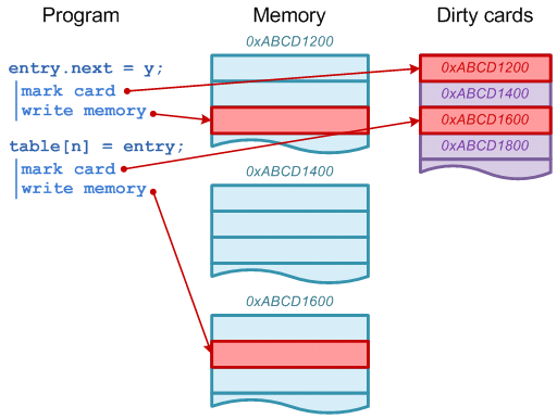
Principle of dirty card write-barrier is very simple. Each time when program modifies reference in memory, it should mark modified memory page as dirty. There is a special card table in JVM and each 512 byte page of memory has associated byte in card table.

Young space collection algorithm

Almost all new objects (there are few exception when new object can be allocated directly in old space) are allocated in Eden space. To be more effective HotSpot is using thread local allocation blocks (TLAB) for allocation of new objects, but TLAB themselves are allocated in Eden. Once Eden becomes full minor GC is triggered. Goal of minor GC is to clear fresh garbage in Eden space. Copy-collection algorithm is used (live objects are copied to another space, and then whole space is marked as free memory). But before start collecting live objects, JVM should find all root references. Root references for minor GC are references from stack and all references from old space.

Normally collection of all reference from old space will require scanning through all objects in old space. That is why we need write-barrier. All objects in young space have been created (or relocated) since last reset of write-barrier, so non-dirty pages cannot have references into young space. This means we can scan only object in dirty pages.

Once initial reference set is collected, dirty cards are reset and JVM starts coping of live objects from Eden and one of survivor spaces into other survivor space. JVM only need to spend time on live objects. Relocating of object also requires updating of references pointing to it.

While JVM is updating references to relocated object, memory pages get marked again, so we can be sure what on next young GC only dirty pages has references to young space.

Finally we have Eden and one survivor space clean (and ready for allocation) and one survivor space filled with objects.

Object promotion

If object is not cleared during young GC it will be eventually copied (promoted) to old space. Promotion occurs in following situations:

• -XX:+AlwaysTenure  makes JVM to promote objects directly to old space instead of survivor  space (survivor spaces are not used in this case).
• once survivor space is full, all remaining live object are relocated directly to old space.
• If object has survived certain number of young space collections, it will be promoted to old space (required number of collections can be adjusted using –XX:MaxTenuringThreshold option and –XX:TargetSurvivorRatio JVM options).

Allocation of new objects in old space

It would be beneficial if we could possibly allocate long lived objects directly in old space. Unfortunately there is no way to instruct JVM to do this for particular object. But there are few cases when object can be allocated directly in old space.

• Option -XX:PretenureSizeThreshold=<n> instructs JVM what all objects larger  than <n> bytes should be allocated directly in old space (though if object size fits TLAB, JVM will allocate it in TLAB and thus young space, so you should also limit TLAB size).
• If object is larger than size of Eden space it also will be allocated in old space.

Unlike application objects, system objects are always allocated by JVM directly in permanent space.

Parallel execution

Most of task during young space collection can be done in parallel. If there are several CPUs available, JVM can utilize them to compress duration of stop-the-world pause during collection. Number of threads can be configured in HotSpot JVM by –XX:ParallelGCTreads= parameter. By default JVM will choose number of thread by number of available CPU. As expected, serial version of collector will ignore this parameter because it can use only one CPU. Using parallel collection reduces time of stop-the-world pause by factor close to number of physical cores.

Time of young GC

Young space collection happens during stop-the-world pause (all non-GC-related threads in JVM are suspended). Wall clock time of stop-the-world pause is very important factor for applications (especially applications requiring fast response time). Parallel execution affects wall clock time of pause but not work effort to be done.

Let’s summarize components of young GC pause. Total pause time can be written as:

T_young = T_{stack_scan} + T_card__scan + T_old__scan+ T_copy ; there T_young is total time of young GC pause, T_{stack_scan} is time to scan root in stacks, T_card__scan is time to scan card table to find dirty pages, T_old__scan  is time to scan roots in old space and T_copy is time to copy live objects (1).

Thread stack are usually very small, so major factors affecting time of young GC is T_card__scan , T_old__scan and T_copy.

Another important parameter is frequency of young GC. Period between young collections is mainly determined by application allocation rate (bytes per second) and size of Eden space.

P_young = S_eden / R_alloc ; there P_young  is period between young GC, S_eden is size of Eden and R_alloc is rate of memory allocations (bytes per second) (2).

T_{stack_scan} – can be considered application specific constant.

T_{card_scan} – is proportional to size of old space. Literally, JVM have to check single byte of table for each 512 bytes of heap (e.g. 8G of heap -> 16m to scan).

T_old__scan  – is proportional to number of dirty cards in old space at the moment of young GC. If we assume that references to young space are distributed randomly in old space, then we can provide following formula for time of old space scanning.

; there S_old is size of old space and D, k_card and n_card are coefficients specific for application (3).

T_copy – is proportional to number of live objects in heap. We can approximate it by formula:

There k_copy is effort to copy object, R_{long_live} is rate of allocation of long lived objects,  

(k_survive usually very small), and k_tenure is a coefficient to approximate aging of object in young space before tenuring (k_tenure ≥ 1) (4).

Now we can analyze how various JVM options may affect time and frequency of young GC.

Size of old space.

Size of old space is affecting T_{card_scan} and T_{old_scan} part of young GC pause time according to formulas above. So we as we are increasing size of old space (read total heap size) time of young GC pauses will grow and it cannot be helped. After certain size of heap (usually 4-8 Gb) time of young collection is dominated by T_{card_scan} (technically T_copy can be even greater than T_{card_scan} , but it usually can be controlled by tuning of other GC options).

HotSpot JVM options:

-Xmx=<n> -Xms=<n>

Size of Eden space 

Period between young GC is proportional to size of Eden. T_copy is also proportional to size of eden but in practice k_survive can be so small that for some applications we can forget about Tcopy. Unfortunately time between young GC will also affect coefficient D in equation (4). Though dependency between D and P_young is very application specific, increasing P_young will increase D and as a consequence T_{scan_old}.

HotSpot JVM options:

-XX:NewSize=<n> -XX:MaxNewSize=<n>

Size of survivor space. 

Size of survivor space puts hard limit of how much objects can stay in young space between collections. Changing size of survivor space may affect k_tenure (or mat not, e.g. if k_tenure is already 1).

HotSpot JVM options:

-XX:SurviorRatio=<n>

Max tenuring threshold and target survivor ratio 

These two JVM options also allow artificially adjust k_tenure.

HotSpot JVM options:

-XX:TargetSurviorRatio=<n>
‑XX:MaxTenuringThreshold=<n>
-XX:+AlwaysTenure
-XX:+NeverTenure

Pretenuring threshold 

For certain applications using pretenuring threshold could reduce k_survive due to allocation of long lived object directly in old space.

HotSpot JVM options:

-XX:PretenureThreshold=<n>

See also

Other articles about garbage collection in this blog

Indexes: RDBMS vs Coherence vs Lucene

Techincal article comparing popular indexing algorithms between RDBMS, data grid (Oracle Coherence) and full text search engine (Lucene).

Most people are familiar with concept of “index” in SQL database. But indexes are widely used far beyond relational databases. There are even dedicated products, like search engines, which are specializing in indexing of data stored elsewhere. This article will give a high level comparison of capabilities and performance aspects of typical indexes in three different types of technologies: SQL database, in-memory-data-grid (Oracle Coherence) and full text search engine (Apache Lucene).

Full text of article is available at GridDynamics blog - http://blog.griddynamics.com/2011/04/indexes-rdbms-vs-coherence-vs-lucene.html

Data Grid Pattern - Snowflake data schema

Evil of distributed joins

Traditionally data grids based solutions are using denormalized data models. Denormalized model allows reducing number of data lookups in storage and achieve low response time. Traditional normalized data models are no good for distributed key/value storages. Main argument against them is requirement to do multiple joins during typical data access operation. If your data are partitioned, joins are becoming prohibitively expensive. You have to join each partition from left join side with each partition on right side thus cost of join grows in quadratic proportion of your number of partitions. 

Even if you can narrow record set before actual join, your data is still may be located on different servers. Each join between partitioned tables will force your data to be moved across network, adding network latency to response time. More joins – more latency accumulated and you will find you out of your allowed response time very soon.
I other words, generally, in grid, you cannot use neither joins, nor normalized data model (though there may always be an exception).

Denormalization is evil

But data denormalization approach is far from perfect. It has its downsides and serious ones. Data redundancy is a side effect of denormalization. Redundancy increase memory consumption and cost of updates. Loosing consistency due to redundancy is another foe. It is a constant battle.

Data warehousing experience

Data warehousing industry has similar challenges to solve. They have huge amounts of data and also have to deal with distributed data storages. And they have an answer to this challenge for some time!

Analytic databases are usually using "snowflake" data model. Snowflake schema has single fact table (in center of schema) and several dimension tables. Size of fact table is huge; sizes of dimension tables are relatively small.

Below are few examples to illustrate snowflake schema.

From financial industry

and from retail

Snowflake data model allows implementing joins across distributed data storage in smart way. While we still want to have fact data to be partitioned across cluster, we can have a full copy of dimension tables on each node executing queries. In other words we may use replication strategy for small dimension table while keeping large fact data partitioned.
Now we can partially execute query using dimensions which are available in local memory of process and then issue single query to fact table. As long as you do not need to join “facts” table with itself of another facts table query execution requires just one network round trip (and if you really need joins between facts wait for next article “Map/Reduce in data grid”).

How can we you utilize snowflake schema with grid middleware?

First we have to decide how we are going to store dimensions tables in memory. We can use in-memory data grid itself or we can use some in-memory database like Hypersonic or H2 database. Grid will support replication of dimension data out of box and natural support for java object, but in memory relational DB will offer better support for queries (e.g. Oracle Coherence does not support any kind of joins even in replicated storage).
Next question is cluster topology, we may replicate dimension data over all nodes or just few of them (query nodes). These query nodes can be either grid peer or remote grid client.
Functional separation between query nodes and data nodes (one storing partitions of facts table) is probably most practical because they have different memory/CPU usage. This way you can tune JVM memory options and scale each tier independently.

Unfortunately this is just a pattern but not built in feature any data grid product I'm aware of. You still have to complete a lot of non trivial engineering to make it work, but this work worth an effort. This pattern allows to use IMDG in cases they denormalization is unable to solve problem, opening new horizons for using of technology.