Showing posts with label performance. Show all posts

Monday, March 11, 2019

Lies, darn lies and sampling bias

Sampling profiling is very powerful technique widely used across various platforms for identifying hot code (execution bottlenecks).

In Java world sampling profiling (thread stack sampling to be precise) is supported by every serious profiler.

While being powerful and very handy in practice, sampling has well known weakness – sampling bias. It is real and well-known problem, though its practical impact is often being over exaggerated.

A picture is worth a thousand of words, so let me jump start with example.

Case 1

Below is a simple snippet of code. This snippet is doing cryptographic hash calculation over a bunch of random strings.

import java.security.MessageDigest;
import java.security.NoSuchAlgorithmException;
import java.util.concurrent.TimeUnit;

public class CryptoBench {

 private static final boolean trackTime = Boolean.getBoolean("trackTime");
 
 public static void main(String[] args) {
  CryptoBench test = new CryptoBench();
  while(true) {
   test.execute();
  }  
 }
 
 public void execute() {
        long N = 5 * 1000 * 1000;
        RandomStringUtils randomStringUtils = new RandomStringUtils();
        long ts = 0,tf = 0;
        long timer1 = 0;
        long timer2 = 0;
        long bs = System.nanoTime();
        for (long i = 0; i < N; i++) {
         ts = trackTime ? System.nanoTime() : 0;
            String text = randomStringUtils.generate();
            tf = trackTime ? System.nanoTime() : 0;
            timer1 += tf - ts;
            ts = tf;
   crypt(text);
   tf = trackTime ? System.nanoTime() : 0;
   timer2 += tf - ts;
   ts = tf;
        }
        long bt = System.nanoTime() - bs;
        System.out.print(String.format("Hash rate: %.2f Mm/s", 0.01 * (N * TimeUnit.SECONDS.toNanos(1) / bt / 10000)));
        if (trackTime) {
         System.out.print(String.format(" | Generation: %.1f %%",  0.1 * (1000 * timer1 / (timer1 + timer2))));
         System.out.print(String.format(" | Hashing: %.1f %%", 0.1 * (1000 * timer2 / (timer1 + timer2))));
        }
        System.out.println();
 }

    public String crypt(String str) {
        if (str == null || str.length() == 0) {
            throw new IllegalArgumentException("String to encrypt cannot be null or zero length");
        }
        StringBuilder hexString = new StringBuilder();
        try {
            MessageDigest md = MessageDigest.getInstance("MD5");
            md.update(str.getBytes());
            byte[] hash = md.digest();
            for (byte aHash : hash) {
                if ((0xff & aHash) < 0x10) {
                    hexString.append("0" + Integer.toHexString((0xFF & aHash)));
                } else {
                    hexString.append(Integer.toHexString(0xFF & aHash));
                }
            }
        } catch (NoSuchAlgorithmException e) {
            e.printStackTrace();
        }
        return hexString.toString();
    }
}
code is available on github

Now let’s use a Visual VM (a profiler bundled with Java 8) and look how much time is actually spent in CryptoBench.crypt() method.

Something in definitely off in screenshot above!

CryptoBench.crypt(), method doing actual cryptography, is attributed only to 33% of execution time.
At same time, CryptoBench.execute() has 67% of self time, and that methods is doing nothing besides calling other methods.

Probably I just need a cooler profiler here. /s

Let’s use Java Flight Recorder for the very same case.
Below is screen shot from Mission Control. 


That looks much better!

CryptoBench.crypt() is now 86% of time our budget. Rest of time code spends in random string generation.
These numbers are looking more belivable to me.

Wait, wait, wait!

Integer.toHexString() is taking as much time as actual MD5 calculation. I cannot belive that.

Numbers are better than ones produced by VisualVM but they are still fishy enough.

Flight recorder is not cool enough for that task! We need really cool profiler! /s

Ok, let me bring some sense into this discrepancy between tools.

We were using thread stack sampling in both tools (Visual VM and Flight Recorder). Though, these tools capture stack traces differently.

Visual VM is actually sampling thread dumps (via thread dump support in JVM). Thread dumps include stack traces for every application thread in JVM, regardless of whatever thread's state is (blocked, sleeping or actually executing code) and this dump is taken atomically. It reflects instant execution state of whole JVM (which is important for deadlock/contention analysis). In practice, that implies short Stop the World pause for each dump. Stop the World pause means safepoint in hotspot JVM. And safepoints brings some nuances.

When Visual VM requests thread dump, JVM notifies threads to suspend execution, but a thread executing Java code wouldn’t stop immediately (unless it is interpreted). The thread would continue to run until next safepoint check where it can suspend itself. Checks cost CPU cycles so they are sparse in JIT generated code.

Checks are placed inside of loops and after method returns. Though, checks are omitted for loops considered “fast” by JIT compiler (typically integer indexed loops). Small methods are aggressively inlined too, hence omiting safepoint check at return. As a consequence, a hot and calculation intensive code may be optimized by JIT into single chunk of machine code which is mostly free of safepoint checks.

If you are lucky, thread dump would show you a line invoking the method containing hot code. With less luck result would be even more misleading.

So in Visual VM call tree we see method CryptoBench.execute() at top of the stack for 66% of samples. If we would be able to see call tree at line number granularity is would be a line calling CryptoBench.crypt() method.

Bad, ugly safepoint bias I’ve caught you red handed! /s

So, how Flight Recorder does sample stacks and why numbers are different?

Flight Recorder sampling doesn’t involve full thread dumps. Instead it freezes threads one by one using OS provided facilities. Once thread is frozen; we can get address of next instruction to be executed out of stack memory area. Address of instruction is converted into line number of java source code via byte code to machine code symbol map. The map is generated during JIT compilation. This is how stack trace is reconstructed.

In case of Flight Recorder safepoint bias does not apply. Though results are still looking inaccurate. Why?

Below is another session with Flight Recorder for the very same code.


Picture is different now.

Integer.toHexString() is just 2.25% of out execution budget which is more trustworthy in my eyes.

Flight Recoder has to resolve memory addresses back to reference of bytecode instruction (which is further transalted into Java source line). Mapping generated by JIT compiler is used for that purpose.

Though compiler is aware that we can see thread stack trace only at safepoints. By default, only safepoint checks are mapped into bytecode instruction indexes. Flight Recorder takes execution address from stack, then it finds next address mapped to Java code in symbol table. In case of aggressive inlining, Flight Recorder can map address to whole wrong point in code.

Though sampling itself is not biased by safepoints, symbol map generated by JIT compiler is.

In second example, I’ve used two JVM options to force more detailed symbol maps to be generated by JIT compler. Options are below.

-XX:+UnlockDiagnosticVMOptions -XX:+DebugNonSafepoints

More accurate, free of bias, symbol map allows Flight Recorder to produce more accurate stack traces.

In our mental model, code is being executed line by line (bytecode instruction by instruction). But complier lumps bunch of methods together and generates single blob of machine code, aggressively reordering operations in the middle of process to make code faster.
Our mental model of line by line execution is totally broken by compiler optimization.

Though, in practice artifacts of operation reordering are not that striking as safepoint bias.

So Java Flight Recorder is cool, Visual VM is not. Should I make this conclusion?

Let me present a counter example.

Case 2

Below is profiling reports from a differnt case.

Now I’m using flame graph generated from data captured by Visual VM and Flight Recorder (with –XX:+DebugNonSafepoints).

Visual VM report 


Flight Recorder report 

Both graphs are showing InflaterInputStream to be a bottleneck. Though Visual VM assesses time spent as 98%, but in Flight Recorder it is just 47%.

Who is right?

Correct answer is 92% (which is approximated using differential analysis).

My heart is broken! Flight Recorder is not a silver bullet. /s

What have gone wrong?

In this example, hot spot was related to JNI overhead involved with calling native code in zlib. It seems like Flight Recorder were unable reconstruct stack trace for certain samples outside of Java code and dropped these samples. Sample population was biased by native code execution. That bias has played against Flight Recorder in this case.

Conclusion

Both profilers are doing that they intended to do. Some sort of bias is natural for almost any kind of sampling.

Each sampling profiler could be categorized by three aspects.

  • Blind spots bias – which samples are excluded from data set collected by profiler.
  • Attractor bias – how samples be attracted to specific discrete points (e.g. safe point).
  • Resolution – unit of code which profiling data is being aggregated to (e.g. method, line number etc).

Below is summary table for sampling methods mentioned in this article.

Blind spot Attractor Resolution
JVM Thread Dump Sampling non-java threads safepoint bias java frames only
Java Flight Recorder non-java code execution CPU pipeline bias
+ code to source mapping skew
java frames only
Java Flight Recorder
+ DebugNonSafepoint
non-java code execution CPU pipeline bias
+ code to source mapping skew
java frames only


Wednesday, May 30, 2018

SJK is learning new tricks

SJK or (Swiss Java Knife) was my secret weapon for firefighting various types of performance problems for long time.

A new version of SJK was released not too long ago and it contains а bunch of new and powerful features I would like to highlight.

ttop contention monitoring

SJK is living it's name by bundling a number of tool into single executable jar. Though, ttop is a likely single most commonly used tool under SJK roof.

ttop is a kind top for threads of JVM process. Besides CPU usage counter (provided by OS) and allocation rate (tracked by JVM), a new thread contention metrics was introduced in recent SJK release.

Thread contention metrics are calculated by JVM, which counts and times when Java threads enters into BLOCKED or WAITING state.

If enabled, SJK is using these metrics to display rates and percentage of time spent in either state.

2018-05-29T14:20:03.382+0300 Process summary 
  process cpu=231.09%
  application cpu=212.78% (user=195.86% sys=16.92%)
  other: cpu=18.31% 
  thread count: 157
  GC time=4.72% (young=4.72%, old=0.00%)
  heap allocation rate 976mb/s
  safe point rate: 6.3 (events/s) avg. safe point pause: 8.24ms
  safe point sync time: 0.07% processing time: 5.09% (wallclock time)
[000180] user=19.40% sys= 0.31% wait=183.6/s(75.77%) block=    0/s( 0.00%) alloc=  110mb/s - hz._hzInstance_2_dev.cached.thread-8
[000094] user=16.92% sys= 0.16% wait=58.50/s(81.54%) block=    0/s( 0.00%) alloc=   94mb/s - hz._hzInstance_3_dev.generic-operation.thread-0
[000057] user=15.05% sys= 0.62% wait=56.91/s(82.35%) block= 0.20/s( 0.01%) alloc=   91mb/s - hz._hzInstance_2_dev.generic-operation.thread-0
[000095] user=15.21% sys= 0.00% wait=55.61/s(82.32%) block= 0.30/s( 0.04%) alloc=   87mb/s - hz._hzInstance_3_dev.generic-operation.thread-1
[000022] user=14.59% sys= 0.00% wait=56.01/s(83.42%) block= 0.30/s( 0.08%) alloc=   86mb/s - hz._hzInstance_1_dev.generic-operation.thread-1
[000058] user=13.97% sys= 0.16% wait=56.91/s(84.13%) block= 0.10/s( 0.02%) alloc=   81mb/s - hz._hzInstance_2_dev.generic-operation.thread-1

An important fact about these metrics is - CPU time + WAITING + BLOCKED should be 100% in ideal world.

In reality, you a likely to see a gap. A few reason why equation above is not holding:

  • GC pauses are freezing thread execution, but not accounted by thread contention monitoring,
  • thread may be waiting for IO operation, but it is not accounted as BLOCKED or WAITING state by JVM,
  • system may starve on CPU resource and thread is waiting for CPU core on OS level (which is also not accounted by JVM).

Contention monitoring is not enabled by default, use -c flag with ttop command to enabled it.

HTML5 based flame graph

SJK was able to produce flame graphs for sometime already. Though, old flame graphs were generated as svg with limited interactivity.

New version offers a new type of flame graphs based on HTML5 and interactive. Right in browser it allows:

  • filtering data by threads,
  • zoom into specific paths or by presence of specific frame,
  • filtering data by thread state (if state information is available).

HTML5 report is 100% self contained file with no dependencies, it can sent it by email and open on any machine. Here is an example of new flame graph you can play right now.

New flame command is used to generate HTML5 flame graphs.

`jstack` dump support

SJK is accepting a number of input data formats for thread sampling data, which is used for flame graphs and other types of performance analysis.

A new format added in 0.10 version is text thread dump formats produced by jstack. Full list of input formats now:

  • SJK native thread sampling format
  • JVisualVM sampling snapshots (.nps)
  • Java Flight Recorder recording (.jfr)
  • jstack produced text thread dumps

Tuesday, October 25, 2016

HotSpot JVM garbage collection options cheat sheet (v4)

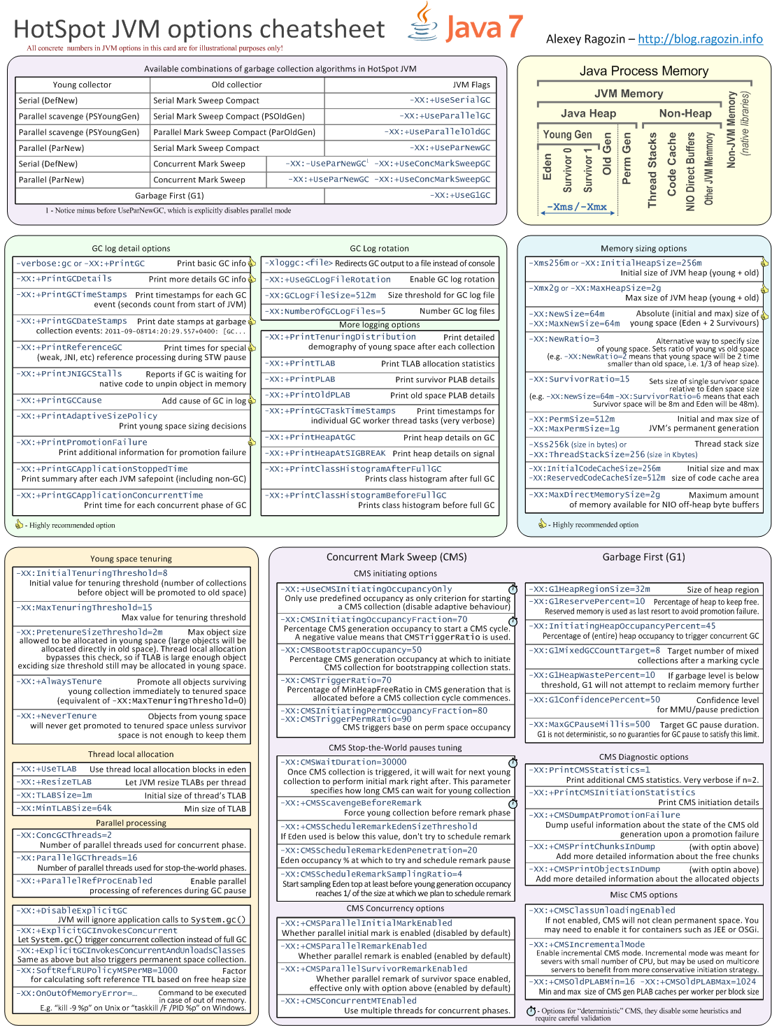
After three years, I have decided to update my GC cheat sheet.

New version finally includes G1 options, thankfully there are not very many of them. There are also few useful options introduced to CMS including parallel inital mark and initiating concurrent cycles by timer.

Finally, I made separate cheat sheet versions for Java 7 and Java 8.

Below are links to PDF versions

Java 8 GC cheat sheet

Java 7 GC cheat sheet

Sunday, January 24, 2016

Flame Graphs Vs. Cold Numbers

Stack trace sampling is very powerful technique for performance troubleshooting. Advantages of stack trace sampling are

  • it doesn't require upfront configuration
  • cost added by sampling is small and controllable
  • it is easy to compare analysis result from different experiments

Unfortunately, tools offered for stack trace analysis by widespread Java profilers are very limited.

Solving performance problem in complex applications (a lot of business logic etc) is one of my regular challenges. Let's assume I have another misbehaving application at my hands. First step would be to localize bottleneck to specific part of stack.

Meet call tree

Call tree is built by digesting large number of stack traces. Each node in tree has a frequency - number of traces passing though this node.

Usually tools allow you to navigate through call tree reconstructed from stack trace population.

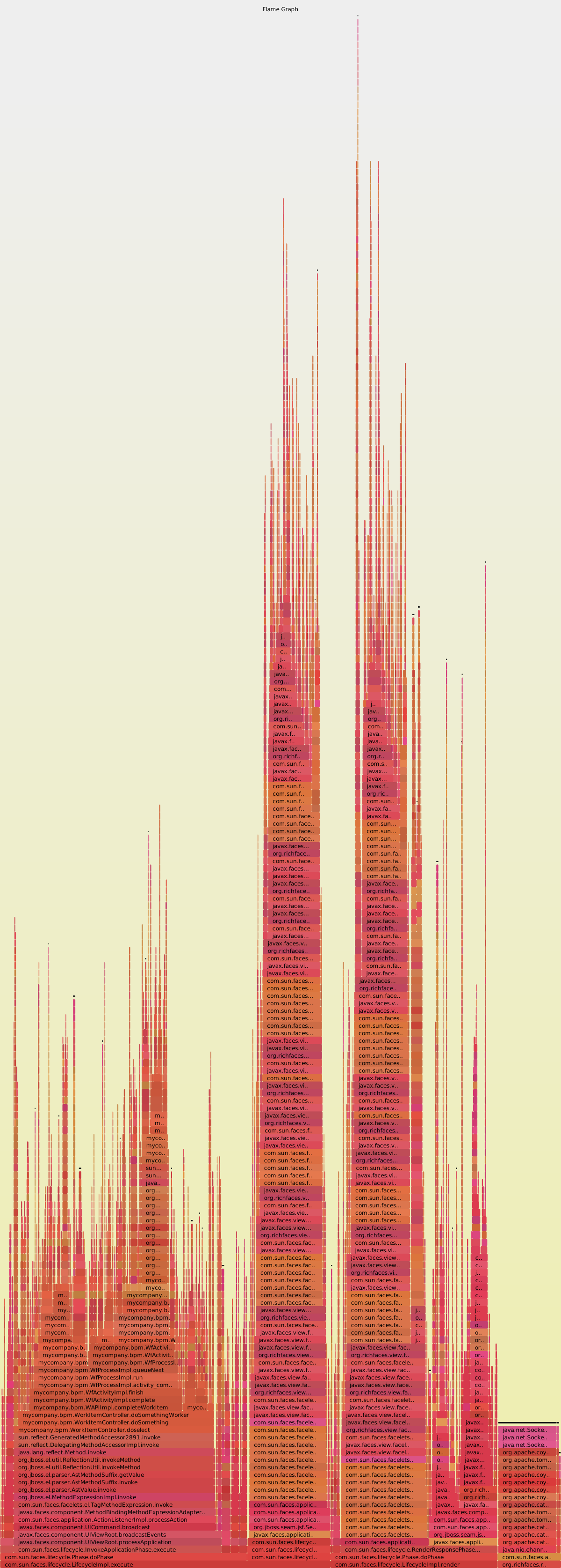
There is also flame graphs visualization (shown at right top of page) which is fancier but is just the same tree.

Looking at these visualization what can I see? - Not too much.

Why? Business logic somewhere in the middle of call tree produces too many branches. Tree beneath business logic is blurred beyond point of usability.

Dissecting call tree

Application is build using frameworks. For the sake of this article, I'm using example based on JBoss, JSF, Seam, Hibernate.

Now, if 13% of traces in our dump contain JDBC we can conclude what 13% of time is spent in JDBC / database calls.
13% is reasonable number, so database is not to blame here.

Let's go down the stack, Hibernate is next layer. Now we need to calculate all traces containing Hibernate classes excluding ones containing JDBC. This way we can attribute traces to particular framework and quickly get a picture where time is spent at runtime.

I didn't find any tool that can do it kind of analysis for me, so I build one for myself few years ago. SJK is my universal Java troubleshooting toolkit.

Below is command doing analysis explained above.

sjk ssa -f tracedump.std  --categorize -tf **.CoyoteAdapter.service -nc
JDBC=**.jdbc 
Hibernate=org.hibernate
"Facelets compile=com.sun.faces.facelets.compiler.Compiler.compile"
"Seam bijection=org.jboss.seam.**.aroundInvoke/!**.proceed"
JSF.execute=com.sun.faces.lifecycle.LifecycleImpl.execute
JSF.render=com.sun.faces.lifecycle.LifecycleImpl.render
Other=**

Below is output of this command.

Total samples    2732050 100.00%
JDBC              405439  14.84%
Hibernate         802932  29.39%
Facelets compile  395784  14.49%
Seam bijection    385491  14.11%
JSF.execute       290355  10.63%
JSF.render        297868  10.90%
Other             154181   5.64%

Well, we clearly see a large amount of time spent in Hibernate. This is very wrong, so it is first candidate for investigation. We also see that a lot of CPU is spent on JSF compilation, though pages should be compiled just once and cached (it turned out to be configuration issue). Actual application logic falls in JFS life cycle calls (execute(), render()). I would be possible to introduce additional category to isolate pure application logic execution time, but looking at numbers, I would say it is not necessary until other problems are solved.

Hibernate is our primary suspect, how to look inside? Let's look at method histogram for traces attributed to Hibernate trimming away all frames up to first Hibernate method call.

Below is command to do this.

sjk ssa -f --histo -tf **!**.jdbc -tt ogr.hibernate

Here is top of histogram produced by command

Trc     (%)  Frm  N  Term    (%)  Frame                                                                                                                                                                                  
699506  87%  699506       0   0%  org.hibernate.internal.SessionImpl.autoFlushIfRequired(SessionImpl.java:1204)                                                                                                          
689370  85%  689370      10   0%  org.hibernate.internal.QueryImpl.list(QueryImpl.java:101)                                                                                                                              
676524  84%  676524       0   0%  org.hibernate.event.internal.DefaultAutoFlushEventListener.onAutoFlush(DefaultAutoFlushEventListener.java:58)                                                                          
675136  84%  675136       0   0%  org.hibernate.internal.SessionImpl.list(SessionImpl.java:1261)                                                                                                                         
573836  71%  573836       4   0%  org.hibernate.ejb.QueryImpl.getResultList(QueryImpl.java:264)                                                                                                                          
550968  68%  550968       1   0%  org.hibernate.event.internal.AbstractFlushingEventListener.flushEverythingToExecutions(AbstractFlushingEventListener.java:99)                                                          
533892  66%  533892     132   0%  org.hibernate.event.internal.AbstractFlushingEventListener.flushEntities(AbstractFlushingEventListener.java:227)                                                                       
381514  47%  381514     882   0%  org.hibernate.event.internal.AbstractVisitor.processEntityPropertyValues(AbstractVisitor.java:76)                                                                                      
271018  33%  271018       0   0%  org.hibernate.event.internal.DefaultFlushEntityEventListener.onFlushEntity(DefaultFlushEntityEventListener.java:161)

Here is our suspect. We spent 87% of Hibernate time in autoFlushIfRequired() call (and JDBC time is already excluded).

Using few commands we have narrowed down one performance bottleneck. Fixing it is another topic though.

In a case, I'm using as example, CPU usage of application were reduced by 10 times. Few problems found and addressed during that case were

  • optimization of Hibernate usage
  • facelets compilation caching were properly configure
  • work around performance bug in Seam framework was implemented
  • JSF layouts were optimized to reduce number of Seam injections / outjections

Limitations of this approach

During statistical analysis of stack traces you deal with wallclock time, you cannot guest real CPU time using this method. If CPU on host is saturated, your number will be skewed by the threads idle time due to CPU starvation.

Normally you can get stack trace only at JVM safepoints. So if some methods are inlined by JIT compiler, they may never appear at trace even if they are really busy. In other words, tip of stack trace may be skewed by JIT effects. Practically, it was never an obstacle for me, but you should be keep in mind possibility of such effect.

What about flame graphs?

Well, despite being not so useful, they look good on presentations. Support for flame graphs was added to SJK recently.

Update

After some time, I've found my self using flame graphs very actively. Yes, for certain situation this type of visualization doesn't make sense, but as a first bird eye look at the problem flame graphs are indispensable.

Monday, October 12, 2015

Does Linux hate Java?

Recently, I have discovered a fancy bug affecting few version of Linux kernel. Without any warnings JVM just hangs in GC pause forever. Root cause is a improper memory access in kernel code. This post by Gil Tene gives a good technical explanation with deep emotional coloring.

While this bug is not JVM specific, there are few other multithreaded processes you can find on typical Linux box.

This recent bug make me remember few other cases there Linux screws Java badly.

Transparent huge pages

Transparent huge pages feature was introduced in 2.6.38 version of kernel. While it was intended to improve performance, a lot of people reports negative effects related to this feature, especially for memory intensive processes such as JVM and some database engines.

  • Oracle - Performance Issues with Transparent Huge Pages
  • Transparent Huge Pages and Hadoop workloads
  • Why TokuDB Hates Transparent Huge Pages
  • Leap seconds bug

    Famous leap second bug in Linux has produced a whole plague across data centers in 2012. Java and MySQL were affected most badly. What a common between Java and MySQL, both are using threads extensively.

    So, Linux, could you be a little more gentle with Java, please ;)

    Tuesday, August 4, 2015

    SJK - missing link in Java profiling tool chain

    Sometimes it just happens. You have a bloated Java application at your hand and it does not perform well. You may have built this application yourself or just got it as it is now. It doesn't matter, thing is - you do not have a slightest idea what is wrong here.

    Java ecosystem have abundance of diagnostic tools (thank for interfaces exposed at JVM itself), but they are mostly focused on some specific narrow kinds of problems. Despite calling themselves intuitive, they assume you have a lot of background knowledge about JVM and profiling techniques. Honestly, even seasoned Java (I'm speaking for myself here) developer can feel lost first time looking at JProfiler, YourKit of Mission Control.

    If you have a performance problem at your hand, first you need is to classify problem: is it in Java or database or somewhere else? is CPU or memory kind of problem? Once you know what kind of problem you have, you can choose next diagnostic approach consciously.

    Are we CPU bound?

    One of first thing you would naturally do is to check CPU usage of your process. OS can show you process CPU usage. Which is useful, but the next question is which threads are consuming it. OS can show you threads usage too, you can even get OS IDs for your Java threads using jstack and correlate them ... manually (sick).

    A simple tool showing CPU usage per Java thread is the thing I wanted badly for the years.

    Surprisingly, all information is already in JMX Threading MBean. All is left is to do trivial math and report per thread CPU usage. So I just did it and ttop command become first in SJK tool set.

    Besides CPU usage JMX have another invaluable metric - per thread allocation counter.

    Collecting information from JMX is safe and can be done on live application instance (in case if you do not have JMX port open, SJK can connect using process ID).

    Below is example of ttop command output.

    2014-10-01T19:27:22.825+0400 Process summary
      process cpu=101.80%
      application cpu=100.50% (user=86.21% sys=14.29%)
      other: cpu=1.30%
      GC cpu=0.00% (young=0.00%, old=0.00%)
      heap allocation rate 123mb/s
      safe point rate: 1.5 (events/s) avg. safe point pause: 0.14ms
      safe point sync time: 0.00% processing time: 0.02% (wallclock time)
    [000037] user=83.66% sys=14.02% alloc=  121mb/s - Proxy:ExtendTcpProxyService1:TcpAcceptor:TcpProcessor
    [000075] user= 0.97% sys= 0.08% alloc=  411kb/s - RMI TCP Connection(35)-10.139.200.51
    [000029] user= 0.61% sys=-0.00% alloc=  697kb/s - Invocation:Management
    [000073] user= 0.49% sys=-0.01% alloc=  343kb/s - RMI TCP Connection(33)-10.128.46.114
    [000023] user= 0.24% sys=-0.01% alloc=   10kb/s - PacketPublisher
    [000022] user= 0.00% sys= 0.10% alloc=   11kb/s - PacketReceiver
    [000072] user= 0.00% sys= 0.07% alloc=   22kb/s - RMI TCP Connection(31)-10.139.207.76
    [000056] user= 0.00% sys= 0.05% alloc=   20kb/s - RMI TCP Connection(25)-10.139.207.76
    [000026] user= 0.12% sys=-0.07% alloc=  2217b/s - Cluster|Member(Id=18, Timestamp=2014-10-01 15:58:3 ...
    [000076] user= 0.00% sys= 0.04% alloc=  6657b/s - JMX server connection timeout 76
    [000021] user= 0.00% sys= 0.03% alloc=   526b/s - PacketListener1P
    [000034] user= 0.00% sys= 0.02% alloc=  1537b/s - Proxy:ExtendTcpProxyService1
    [000049] user= 0.00% sys= 0.02% alloc=  6011b/s - JMX server connection timeout 49
    [000032] user= 0.00% sys= 0.01% alloc=     0b/s - DistributedCache
    

    Besides CPU and allocation, it also collect "true" GC usage and safe point statistics. Later two metrics are not available via JMX so they are available only for process ID connections.

    CPU usage picture will give you good insight what to do next: should you profile your Java hot spots or all time is spent waiting result from DB.

    Garbage analysis

    Another common class of Java problems is related to garbage collection. If this is a case GC logs is first place to look at.

    Do you have them enabled? If not, that is not a big deal, you can enable GC logging on running JVM process using jinfo command. You can also use SJK's gc command to peek GC activity for your java process (it is not as full as GC logs tough).

    If GC logs confirm what GC is causing you problems, next step is to identify where that garbage comes from.

    Commercial profilers are good at memory profiling, but this kind of analysis slows down target application dramatically.

    Mission Control stands out of pack here, it can profile by sampling TLAB allocation failures. This technique is cheap and generally produce good results, though it is inherently biased and may mislead you sometimes.

    For long time jmap and class histogram were main memory profiling instrument for me. Class histogram is simple and accurate.

    In SJK] toolset, I have augmented vanila jmap command a little to make it more useful (SJK's [hh command).

    Beware that jmap (and thus hh command) required Stop the World pause on target JVM while heap is being walked, so it may not be a good idea to execute it against live application under load.

    Dead heap histogram is calculated as difference between object population before and after forced GC (using jmap class histogram command under hood).

    Dead young heap histogram enforces full GC then wait 10 seconds (by default) then produce dead object histogram by technique describe above. Thus you see a summary freshly allocated garbage.

    This methods cannot not tell you where in your code that garbage was allocated (this is job for Mission Control et al ). Though, if you know that is your top garbage objects, you may already know there they are allocated.

    SJK have a few more tools but these two ttop and hh are always in front lines when I need to tackle another performance related problem.

    Wednesday, February 11, 2015

    Binary search - is it still most optimal?

    If you have a sorted collection of elements, how would you find index of specific value?
    "Binary search" is likely to be your answer.
    Algorithms theory is teaching us what binary search is most optimal algorithm for this task with log(N) complexity.
    Well, hash table can do better, if you need to find key by exact match. In many cases, though, you have reasons to have your collection sorted, not hashed.

    On my job, I'm working on sophisticated in-memory database tailored for streaming data processing. We have a lot of places where we deal with sorted collection of integers (data row references, etc).

    Algorithms theory is good, but in reality there are things like cache hierarchy, branch prediction, super scalar execution which may skew performance at edge cases.

    Question is - where lie borders between reality ruled by CPU quirks and lawful space of classic algorithms theory?

    If you have a doubt - do an experiment.

    Experiment is simple: I'm generating a large number of sorted arrays of 32 bit integers. When I search random key in random array multiple times. In each experiment average size of array is fixed. Large number of arrays used to ensure cold memory access. Average time search time is measured.

    All code written in Java and measured using JMH tool.

    Participants are

    • Binary search - java.util.Arrays.binarySearch()
    • Linear search - simple loop over array until key is found
    • Linear search 2 - looping over every second element in array, if greater key is found, check i - 1 index too

    X axis is average array length
    Y axis is average time of single search in microseconds
    Measurments have been done on 3 different types CPU.

    Results speak for themselves.

    I was surprised a little, as I were expecting binary search to outperform linear at length of 32 or 64, but it seems that modern processors are very good at optimizing linear memory access.

    Provided that 8 - 128 is a practical range for BTree like structures, I will likely to reconsider some of data structures used in our database.

    Tuesday, October 29, 2013

    JVM deep dive at HighLoad++ 2013 (Moscow)

    Today was speaking at HighLoad++ 2013 Moscow. I had two presentation covering deep internals of JVM. One about JIT compilation and other concerning pauseless garbage collection algorithms.

    Slide decks are below (in Russian)

    Tuesday, September 10, 2013

    Coherence 101 - EntryProcessor traffic amplification

    Oracle Coherence data grid has a powerful tool for inplace data manipulation - EntryProcessor. Using entry processor you can get reasonable atomicity guarantees without locks or transactions (and without drastic performance fees associated).

    One good example of entry processor would be built-in ConditionalPut processor, which will verify certain condition before overriding value. This, in turn, could be used for implementing optimistic locking and other patterns.

    ConditionalPut could accept only one value, but ConditionalPutAll processor is also available. ConditionalPutAll accepts a map of key/values. Using it, we can update multiple cache entries with single call to NamedCache API.

    But there is one caveat.

    We have placed values for all keys in single map instance inside of entry processor object. On the other side, in distributed cache keys are distributed across different processes.
    How right values would be transferred to right keys?

    Answer is simple - every node, owning at least one of keys to be updated, will receive a copy of whole map of values.
    In other words, in mid size cluster (i.e. 20 nodes) you may actually transfer 20 times more data over network than really needed.

    Modern networks are quite good and you may not notice this traffic amplification effect for some time (as long as you network bandwidth can handle it). But once traffic has reached network limit things are starting to break apart.

    Coherence TCMP protocol is very aggressive at grabbing as much of network bandwidth as it can, so other communications protocols will likely perish first.
    JDBC connections are likely victim of bandwidth shortage.
    Coherence*Extend connection may also suffer (it is using TCP) and proxy nodes may start to fail in unusual ways (e.g. with OutOfMemoryError due transmission backlog overflow).

    This problem may be hard to diagnose. TCP is much more vulnerable to bandwidth shortage and you will be kept distracted with TCP communication problems while root cause is excessive TCMP cluster traffic.

    Monitoring TCMP statistics (available via MBean) could give you an insight about network bandwidth consumption by TCMP and network health and help to find root cause.

    Isolating TCMP in separate switch is also a good practice, BTW

    But how to fix it?

    Manual data splitting

    Simple solution is to split keys set by owning nodes, and then invoke entry processor for each subset individually. Coherence API allows you to find node owning particular key.
    This approach is far from ideal though:

    • it will not work for Extend clients,
    • you either have to process all subset sequentially or use threads to do several parallel calls to Coherence API,
    • splitting of key set complicates application logic.
    Triggers

    Another option is relocating your logic from entry processor to trigger and replacing invokeAll() by putAll() (putAll() does not suffer from traffic amplification). This solution is fairly good and fast, but has certain drawbacks too:

    • it is less transparent (put() is not just put() now),
    • trigger is configured once for all cache operations (not just one putAll() call),
    • you can only have one trigger and it should handle all your data update needs.
    Synthetic data keys

    Finally you can use DataSplittingProcessor from CohKit project. This utility class is using virtual cache keys to transfer data associated with keys, then it is using backing map API to access real entries.

    This solution has its PROs and CONs too:

    • good drop-in replacement for ConditionalPutAll and alike,
    • prone to deadlocks if running concurrently with other bulk updates (it is partially mitigated by sorting keys before locking).

    Choosing right solution

    In practice I was using all three technique listed above.

    Sometimes triggers fit overall cache design quite good.
    Sometimes manual data split has its advantages.
    And sometimes DataSplittingProcessor is just right remedy for existing entry processors.

    Monday, September 9, 2013

    SJK (JVM diagnostic/troubleshoting tools) is learning new tricks.

    SJK is small command line tool implementing number of helpful commands for JMV troubleshooting. Internally SJK is using same diagnostic APIs as standard JDK tools (e.g. jps, jstack, jmap, jconsole).

    Recently I've made few noteworthy additions to SJK package and would like to announce them here.

    Memory allocation rates for Java threads

    ttop command now displays memory allocation per thread and cumulative memory allocation for whole JVM process.
    Memory allocation rate is key information for GC tuning, in past I was using GC log to derive these numbers. On contrast, per thread allocation counters give you more precise information in real time.
    Process allocation rate is calculated by aggregating thread allocation rate.

    more details about ttop

    Support for remote JMX connections

    Historically SJK were using PID to connect to JVM's MBean server. Using PID does not require you to explicitly enable JMX in JVM's command line and offers you OS level security.
    Sometime you already have JMX port up and running (e.g. for other monitoring tools) and connection using host and port is more convenient.
    Now all JVM based commands (ttop, gcrep, mx, mxdump) support socket based JMX connections (with optional user/password security).

    Invoking arbitrary MBean operation

    New command (mx) allows to get/set arbitrary MBean attributes and call arbitrary MBean operations.
    This one is paralytically useful for scripting (I didn't find to invoke operation for custom MBean from command line, so I have added it to SJK).

    more details about ttop

    Code and binaries are available at GitHub
    https://github.com/aragozin/jvm-tools

    Sunday, July 28, 2013

    Java GC in Numbers - Compressed OOPs

    Compressed OOPs (OOP – ordinary object pointer) is a technique reducing size of Java object in 64 bit environments. HotSpot wiki has a good article explaining details. Downside of this technique is what address uncompressing is required before accessing memory referenced by compressed OOPs. Instruction set (e.g. x86) may support such addressing type directly, but still, additional arithmetic would affect processing pipeline of CPU.

    Young GC involves a lot of reference walking, so its time is expected to be affected by OOPs compression.

    In this article, I’m comparing young GC pause time for 64 bit HotSpot JVM with and without OOPs compression. Methodic from previous article is used and benchmark code is available at github. There is one caveat though. With compressed OOPs size of object is smaller and same amount of heap could accommodate more objects. Benchmark is autoscaling number of entries to fill heap based entry footprint and old space size, thus with fixed old space size experiments with compression enabled have to deal with slightly larger number of objects (entry footprints are 288 uncompressed and 246 compressed).

    Chart below shows absolute young GC pause times.

    As you can see, compressed case is consistently slower, which is not a surprise.

    Another char is showing relative difference between two cases (compressed GC pause mean / uncompressed GC pause mean for same case).

    Fluctuating line suggests that I should probably increase number of runs for each data points. But, let’s try to make some conclusion from what we have.

    For heaps below 4GiB JVM is using special strategy (32 address could be used without uncompressing in this case). This difference is visible from chart (please note that point with 4GiB of old space, means that total heap size is above 4GiB and this optimization is inapplicable).

    Above 4 GiB we see 10-30% increase in pause times. You should also not to forget that compressed case have to deal with 17% more data.

    Conclusions

    Using compressed OOPs affects young GC pause time which is not a surprise (especially taking increase amount of data). Using compression for heaps below 4GiB seems to be a total win, for larger heaps it seems to be reasonable price for increase capacity.

    But main conclusion is that experiment has not revealed any surprises neither bad nor good ones. This may be not very exciting but is useful information anyway.

    Thursday, July 11, 2013

    Coherence 101, Filters performance and indexing

    In this post, I would like to share some knowledge about optimizing indexes in Oracle Coherence.

    Normally you should not abuse queering features of your data grid and, hence, you are unlikely to ever need to tune indexing/queering (besides choosing which indexes to create). But sometimes, you really need to squeeze as much performance as you can from your filter based operations. If it is your case, then few tricks described below may be helpful.

    Extractor used to add index, should be "equal" to extractor used in filter

    You are probably aware of this fact, but it is of critical importance and repeating this one more time will not do any harm. All query planning in Coherence relies on matching (using equals() method) of extractors used in index and filter.

    Typical mistakes you could do here:

    • Use semantically equivalent, but different types of extractors (e.g. ReflectionExtractor and ChainedExtractor may extract exactly same attribute, but they will not be equal in Java sense).
    • Use custom extractor classes without implementing equals() and hashCode().
    • Mixing reflection based and POF based extractors.

    In all cases above, your code will work, but index will not be used.

    Indexing attributes with low-cardinality

    Sometimes your query may include criterion for low-cardinality attribute. Not indexing this attribute will cause deserialization of all candidate entries to check attribute value.

    Deserialization is something you really want to avoid in Coherence cluster under heavy load. Besides being CPU consuming, deserialization will produce a lot of garbage, risking to bringing you GC out of balance.

    Adding index may bring another risk though. If you put your predicates in wrong order, such index may only slow down query.

    Below is result of simple benchmark. I was using 2 Coherence storage nodes and 1000000 as data set. Ticker predicate is matching 1000 objects, and side predicate matching 500000. EqualsFilter and AndFilter were used to build query. Execution time of count aggregator was measured.

    Tests were run on my laptop, so absolute numbers are not important (and not statistically sound to be honest).

    Without indexes
    • side & ticker -- 5780 ms
    • ticker & side -- 5687 ms
    Index by ticker
    • side & ticker -- 66 ms
    • ticker & side -- 66 ms
    Both ticker and side indexed
    • side & ticker -- 496 ms
    • ticker & side -- 10 ms

    As you can see, if you are unlucky and your query is not in right order, adding index may actually harm query performance.

    There is a trick to protect you in this case. NoIndexFilter is a filter wrapper, which disables inverted index lookup for nested index. Forward map of index remains accessible, so testing attribute value will not require desrialization.

    Both ticker and side indexed
    • no_index(side) & ticker -- 17 ms
    • ticker & no_index(side) -- 18 ms

    As you can see, it takes some toll on "good query", but negates effect of "wrong order of predicates". You can also see that it is still 3 times faster than case where "side" was not indexed.

    Exploiting composite indexes

    You can make query above even more faster if you really need to.

    Normally, with Coherence, you do not use composite indexes (instead you are indexing attributes individually). Creation of composite index is possible, but you will have to use specially composed queries to exploit composite index.

    Code to add composite index will look like

    ValueExtractor[] ve = {
        new ReflectionExtractor("getTicker"),
        new ReflectionExtractor("getSide")          
    };
    MultiExtractor me = new MultiExtractor(ve);
    cache.addIndex(me, false, null);
    

    and filter exploiting it will look like

    ValueExtractor[] ve = {
        new ReflectionExtractor("getTicker"),
        new ReflectionExtractor("getSide")          
    };
    MultiExtractor me = new MultiExtractor(ve);
    EqualsFilter composite = new EqualsFilter(me, Arrays.asList(ticker, side));
    

    Below are results compared with traditional index/query.

    Without indexes
    • ticker & side -- 5687 ms
    • composite -- 5998 ms
    All Indexes
    • ticker & side -- 11 ms
    • composite -- 3 ms

    Composite index is awkward to use, but, if it matches your case, you can get significant performance gain.

    Few more links

    That is it, for this post. You can also take a look at my slide deck from one of London Coherence SIGs, it explains few more advanced topics about indexes in Oracle Coherence.

    Friday, June 14, 2013

    Java GC in Numbers – Parallel Young Collection

    This is a first articles in series, where I would like to study effect of various HotSpot JVM options on duration of STW pauses associated with garbage collection.

    This article will study how number of parallel threads affects duration of young collection Stop-the-World pause. HotSpot JVM has several young GC algorithms. My experiments are covering following combinations:

  • Serial young (DefNew), Mark Sweep Compact old
  • Parallel young (ParNew), Mark Sweep Compact old
  • Serial young (DefNew), Concurrent Mark Sweep old
  • Parallel young (ParNew), Concurrent Mark Sweep old
  • There is also PSNew (Parallel Scavenge) algorithm similar to ParNew, but it cannot be used together with Concurrent Mark Sweep (CMS), so I have ignored it.

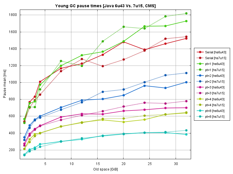
    In experiments, I was using synthetic benchmark producing evenly distributed load on memory subsystem. Size of young generation was same for all experiments (64MiB). Two versions of HotSpot JVM were used: JDK 6u43 (VM 20.14-b01) and JDK 7u15 (VM 23.7-b01).

    Test box was equipped with two 12 core x 2 hardware threads CPUs (totaling in 48 hardware threads).

    Mark Sweep Compact

    Mark Sweep Compact is prone to regular full GCs, so it is not a choice for pause sensitive applications. But it shares same young collection algorithms/code with concurrent collector and produces less noisy results, so I added to better understand concurrent case.

    Difference between single thread case and 48 thread case is significant so number are present in two graphics.

    Note worthy (not surprising though), that serial algorithm performs slightly better than parallel with one thread. Discrepancy between Java 6 and Java 7 is also interesting, but I have no ideas now to explain that.

    From graphics above you can get an idea that more threads is better, but it is not obvious how exactly better. Graphics below show effective parallelization (8 thread case is taken as base value, because smaller numbers of threads are producing fairly noisy results).

    You can see almost linear parallelization up to 16 threads. It is also worth to note, that 48 threads are considerably faster that 24 even though there are only 24 physical cores. Effect of parallelization is slightly better for larger heap sizes.

    Concurrent Mark Sweep

    Concurrent Mark Sweep is a collector used for pause sensitive applications and young collection pause time is something that you probably really care if you have consciously chosen CMS. Same hardware and same benchmark were used.
    Results are below.

    Compared to Mark Sweep Compact, concurrent algorithm is producing much noisy results (especially for small number of threads).

    Java 7 is systematically showing worse performance compared to Java 6, not too much though.

    Parallelization diagrams, show us same picture - linear scalability, which degrades with greater number of threads (experiment conditions is slightly different for CMS and MSC cases, so direct comparison of these diagrams is not correct).

    Conclusions

    Tests have confirmed that parallel young collection algorithms in HotSpot JVM scales extremely well by number of CPU cores. Having a lot of CPU cores on server will help you greatly with JVM Stop-the-World pauses.

    Source code

    Source code used for benchmarking and its description is available at GitHub.
    github.com/aragozin/jvm-tools/tree/master/ygc-bench

    Tuesday, December 4, 2012

    Coherence 101, Beware of cache listeners

    Cache events facility is a quite useful feature of Oracle Coherence. For example, continuous queries and near cache features are build on top of cache event system.
    Unfortunately it could be also abused easily. In particular, they are noticeably bad at scale unless you are very careful.
    Please note. This article is covering only partitioned cache topology (distributed cache scheme).

    Client side map listeners

    UPDATE: I was very wrong in my previous description of client side synchronous map listeners. Section below was rewritten to reflect more accurate picture.

    Client side map listeners are usually added via NamedCache API. They typically receive events from caches hosted on remote JVMs (storage nodes). But regardless of whenever cache event is produced at remote or local JVM, Coherence will deliver it to listeners using dedicated event dispatch thread (or service thread itself for listeners marked as synchronous).

    Each cache service has only one event dispatch thread, and it could easily become a bottle neck, limiting speed of cache event processing on client.

    Few tips to mitigate this design aspect are below.

    • Do not do anything time consuming in listener itself, offload processing to other thread instead.
    • Be careful with synchronization – avoid lock contention in listener code.
    • When event hits your listener, its data are still in binary form. To avoid deserialization cost, do not access key or value in event dispatch thread, instead pass reference to map event object to own processing thread (or thread pool).

    Last advice may not be intuitive, but deserialization of map event in Coherence’s event dispatch thread often becomes a bottleneck slowing down event processing rate.

    Synchronous and normal map listeners

    There is a marker interface SynchronousListener in com.tangosol.util package.
    You could implement it in your map listener. But this wouldn’t make map event delivery to your listener synchronous with cache operation (as you may think), instead it would affect in which thread your listener is invoked.

    Normal listeners are invoked in event dispatch thread.

    “Synchronous” listeners would be invoked in service thread

    What are the differences?

    • Imagine you have near cache and you are using entry processor to update entry. If cache event would be processed in event dispatch thread, data in near cache may remain stale for short time between entry processor call have returned, but event is not processed yet.
      Using of synchronous listeners would solve this, because event would be guaranteed to be processed before processing response message from entry processor invocation.
    • Time consuming custom map listeners could slow down event dispatch thread increasing event delays. This would affect Coherence build-in facilities such as near caches and CQC would be affected because they use synchronous listeners internally - you can consider it extra level of protection from misbehaving developer :)

    But let me stress it again, for any type of listener events are delivered asynchronously relative to other cluster nodes.

    Backing map listeners

    Backing map listeners are used less often (but being abused more frequently). Backing map listeners are usually configured via XML cache configuration and work on storage side.
    On storage side, Coherence could use pool of worker threads to perform operations in parallel. You may assume that you backing map listener would also be invoked in parallel …
    … but that is wrong. Backing map listener could process one map event at time for given cache, regardless of thread pool size.
    First time, I was also surprised by such behavior. This is not fundamental limitation of Coherence, but all out-of-box variations of backing map use cache global lock to dispatch map event. Even for partitioned backing map Coherence will use ObservableSplittingBackingMap wrapper which is, again, using global lock.
    So, if you are using backing map listeners, be aware of that limitation. Live object pattern also relay on backing mapping listener and thus limited by this scalability constraint.

    Map triggers

    Fortunately map triggers work as a part of cache update transaction on cache service level. In other words map trigger would not harm performance more than entry processors do.
    One possible workaround for baking map listeners concurrency issue could be invocation of map listener from map trigger.

    Friday, February 17, 2012

    POF serialization, beware of arrays

    As you may have experienced yourself, object marshaling/serialization often lays on performance critical path in distributed system (especially in Java). Default Java serialization is almost always is a poor choice, countless alternatives was developed to replace it. POF (portable object format) is binary object serialization format which was developed by Oracle Coherence team with both cross platform and efficiency in mind (POF can be compared to Thrift or ProtoBuf). While being compact and efficient POF is also offering advanced features such as access to specific attributes of object without deserializing whole thing.

    But sometime avoiding deserialization may be more expensive than deserialization itself. Below is a short story of my experience worth sharing.

    Recently, I was working on Coherence based solution. After another set code changes, automatic test has shown sudden performance degradation. One of aspect of change set was replacing reflection based filters with ones using PofExtractor. Surprisingly, times of operations which were relying on affected filters have increased about 20 times! While PofExtractors are not always faster compared to ReflectionExtractors in my practice, 20 times slowdown seems to be totally unreasonable. Anyway, switch to PofExtractor was made to avoid classpath dependency, so switching back to ReflectionExtractor was not an option.
    Profiling session have showing interesting results:
    • objects were never completely deserialezed (as expected with PofExtractor),
    • filter execution indeed was a bottleneck,
    • more targeted profiling have identified method PofHelper.skipUniformValue() as a hot spot.
    While PofHelper.skipUniformValue() is expected to be heavy duty method (it is used to parse POF binary stream seeking attribute to be extracted), it was eating unproportionally large amount of CPU. Instrumentation profiling have revealed one more fact - few thousands of calls to skipUniformValue() have been made for each call to PofExtractor.extractFromEntry().

    Well, that could explain HOW code gets slow, but questions are WHY and how to fix it.

    Object, I was working with in application, were mostly wrapper around a chunk of data in proprietary encoded binary format. Few attributes were extracted and stored as fields of java objects, but larges part of object was a single chunk of binary data. This chunk were stored as byte[] in Java and written using writeByteArray() in POF stream. There is another method suitable for this task writeBinary(), but using writeByteArray() just feels more convent. That was a key mistake.

    POF array vs. binary

    POF can encode numbers using variable length format, writeByteArray() encodes byte[] as an array of variable length objects. Well actually they are all exactly one byte at length, but generic POF decode still inspects each byte to calculate array length (and for each byte it would be calling skipUniformValue() which is huge method with switch case for every possible POF data type) . On contrary, writeBinary()writes opaque blob, so parser just reads its size and skips it in single operation.
    I have replaced writeByteArray() with writeBinary() (you may also want to replace read code, but it is not necessary readByteArray()can parse Binary from stream and convert it byte[] for you). It have solved problem.

    Below is comparison of extractor times with various amounts of binary data inside object, using 2 versions of serialization.
    Please mind difference in scale between diagrams, it is an order of magnitude!

    Summary

    Ok, use writeBinary() will help you with byte arrays, but what if you need to store float[] or other array type?
    If arrays are not large it is ok, but if they are, then you should avoid use of PofExtractors, use normal extractors instead.

    I hope this performance issue will be fixed eventually,
    but until it is fixed,
    beware of arrays in your POF objects!

    Sunday, December 4, 2011

    Garbage collection in HotSpot JVM


    In this blog you may find few in-depth articles related to garbage collection in Oracle's HotSpot and other JVMs. But if you a novice in field of garbage collection, you may feel lost due to level of details. So I decided that high level overview of GC modes in HotSpot would add nicely to existing fairly detailed content.

    Foreword

    Java (and dominating majority of other modern languages) features automatic memory management aka garbage collection. Once instance of object becomes unreachable from executing program, it is classified as garbage and, eventually, its memory should be added to free pool.
    One of simplest approaches to automatic memory management is reference counting. But it has serious limitation though, inability to handle cyclic links in object graph.
    If we want to find all effectively unreachable objects, the only way is to find all reachable via recursive object graph traversing. It may sound like a complicated task and it really is.
    Garbage collection in modern JVMs including Oracle's HotSpot is a result of lengthy evolution. Huge amounts  hard work was put into them, to make them as efficient as they is now. Of cause they may have limitations, deficiencies but in most time this due to tradeoffs which was made for reason. So, please think twice before blaming JVM garbage collector being slow or stupid. Most likely you just underestimating complexity of its work.
    Ok, now, let me get straight to garbage collection in HotSpot JVM circa 2011.

    HotSpot JVM circa 2011

    HotSpot has several GC modes. Modes are controlled with JVM command line options.  Default GC mode depends on JVM version, client/server mode of JVM and hardware you are running on (JVM distinguish server and desktop grade hardware by set of heuristics).

    Serial GC

    JVM switch: -XX:+UseSerialGC
    Serial GC is generational garage collection algorithm (if you wander what generation means, read this article).
    Actually all GC modes in HotSpot are using generational approach, so won't repeat it for every GC mode.
    Young collection is a copy collection. Old space is collected using an implementation of mark/sweep/compact (MSC) algorithm. Both, young and old, collections require stop-the-world (STW) pause and, as name suggests, are executed by single thread. During old space collection, all live objects are moved to beginning of space. This allows JVM to return unused memory to OS.

    If you enable GC logging by -XX:+PrintGCDetails you will see following indicators of GC pauses in log:
    Young collection
    41.614 [GC 41.614: [DefNew: 130716K->7953K(138240K), 0.0525908 secs] 890546K->771614K(906240K), 0.0527947 secs] [Times: user=0.05 sys=0.00, real=0.05 secs]
    Full (young + old + perm) collection
    41.908 [GC 41.908: [DefNew: 130833K->130833K(138240K), 0.0000257 secs]41.909: [Tenured: 763660K->648667K(768000K), 1.4323505 secs] 894494K->648667K(906240K), [Perm : 1850K->1850K(12288K)], 1.4326801 secs] [Times: user=1.42 sys=0.00, real=1.43 secs]

    Parallel scavenge

    JVM switch: -XX:+UseParallelGC
    Some phases of garbage collection could be naturally parallelized between multiple threads. Parallel processing can reduce time required for GC and thus STW pause duration by keeping multiple physical CPU cores busy. Adoption of multiprocessor/multicore hardware have made parallelization of GC a must for modern VM.
    Parallel scavenge GC mode is using parallel implementation of young collection algorithm. Old space is still collected by one thread. Thus, using this mode may shorten young collection pauses (which are more frequent), but still suffers from long full collection freezes.

    Log output samples for parallel scavenge.
    Young collection
    59.821: [GC [PSYoungGen: 147904K->4783K(148288K)] 907842K->769258K(916288K), 0.2382801 secs] [Times: user=0.31 sys=0.00, real=0.24 secs]
    Full collection
    60.060: [Full GC [PSYoungGen: 4783K->0K(148288K)] [PSOldGen: 764475K->660316K(768000K)] 769258K->660316K(916288K) [PSPermGen: 1850K->1850K(12288K)], 1.2817061 secs] [Times: user=1.26 sys=0.00, real=1.28 secs]

    Parallel old GC

    JVM switch: -XX:+UseParallelOldGC
    This mode is a incremental improvement over parallel scavenge mode. It adds parallel processing (parallel mark-sweep-compact (MSC) algorithm) for old space collection. Young space is using same algorithm as mode above. Old space collection still requires quite long STW pause, but now multiple cores could be employed to make it shorter. Unlike serial MSC, parallel version does not create single continuous free memory region at the end of heap, so JVM cannot return memory to OS after full GC in this mode.

    Log output samples for parallel old GC.
    Young collection
    65.411: [GC [PSYoungGen: 147878K->5434K(144576K)] 908129K->770314K(912576K), 0.2734699 secs] [Times: user=0.41 sys=0.00, real=0.27 secs]
    Full collection
    65.685: [Full GC [PSYoungGen: 5434K->0K(144576K)] [ParOldGen: 764879K->623094K(768000K)] 770314K->623094K(912576K) [PSPermGen: 1850K->1849K(12288K)], 2.5954844 secs] [Times: user=3.95 sys=0.03, real=2.60 secs]

    Adaptive size policy

    JVM switch: -XX:+UseAdaptiveSizePolicy
    This is a special mode of parallel scavenge collector in which it can dynamically adjust configuration of young space to adapt for an application. IMHO it does not bring much benefits. Never seriously tried to use this option.

    Concurrent mark sweep

    JVM switch: -XX:+UseConcMarkSweepGC
    While collectors above are generally called throughput collectors. Concurrent mark sweep (CMS) is low pause collector. It is designed to minimize stop-the-world JVM pauses and thus keep application responsive. For young space collection it may use either serial copy collector or parallel one (parallel alhorithm is similar to algorithm in parallel scavenge mode, but they are two totally different code bases and they may use slightly different configuration options, e.g. adaptive size policy is not implemented for CMS).
    Old (and if enabled permanent) space a collected by mostly concurrently. As name suggests CMS  is mark sweep algorithm (notice lack of compact in its name). CMS requires only two short pauses during each old space collection cycle. But unlike its stop-the-world counterparts, CMS cannot do compaction (relocate objects in memory) and this makes it prone to fragmentation. CMS is using some tricks to fight fragmentation, but it is still a threat.
    If concurrent collector fails to reclaim memory fast enough to keep with application needs, JVM will fall back to serial stop-the-world mark- sweep-compact algorithm to defragment (and compact) old space (notice serial word, usually such pause would be 50-500 times longer than normal CMS pause).

    Log output samples for CMS.
    Young collection
    613.154: [GC 13.154: [DefNew: 130821K->8230K(138240K), 0.0507238 secs] 507428K->388797K(906240K), 0.0509611 secs] [Times: user=0.06 sys=0.00, real=0.05 secs]
    Concurrent old space collection
    13.433: [GC [1 CMS-initial-mark: 384529K(768000K)] 395044K(906240K), 0.0045952 secs] [Times: user=0.02 sys=0.00, real=0.01 secs]
    13.438: [CMS-concurrent-mark-start]
    ...
    14.345: [CMS-concurrent-mark: 0.412/0.907 secs] [Times: user=1.20 sys=0.00, real=0.91 secs]
    14.345: [CMS-concurrent-preclean-start]
    14.366: [CMS-concurrent-preclean: 0.020/0.021 secs] [Times: user=0.03 sys=0.00, real=0.02 secs]
    14.366: [CMS-concurrent-abortable-preclean-start]
    ...
    14.707: [CMS-concurrent-abortable-preclean: 0.064/0.340 secs] [Times: user=0.36 sys=0.02, real=0.34 secs]
    14.707: [GC[YG occupancy: 77441 K (138240 K)]14.708: [Rescan (non-parallel) 14.708: [grey object rescan, 0.0058016 secs]14.714: [root rescan, 0.0424011 secs], 0.0485593 secs]14.756: [weak refs processing, 0.0000109 secs] [1 CMS-remark: 404346K(768000K)] 481787K(906240K), 0.0487607 secs] [Times: user=0.05 sys=0.00, real=0.05 secs]
    14.756: [CMS-concurrent-sweep-start]
    ...
    14.927: [CMS-concurrent-sweep: 0.116/0.171 secs] [Times: user=0.23 sys=0.02, real=0.17 secs]
    14.927: [CMS-concurrent-reset-start]
    14.953: [CMS-concurrent-reset: 0.026/0.026 secs] [Times: user=0.05 sys=0.00, real=0.03 secs]
    Times marked with green are times of concurrent phases – CMS do its work in parallel with application. You can find out more about CMS pauses here.
    CMS failure and fallback to mark-sweep-compact
    557.079: [GC 557.079: [DefNew557.097: [CMS-concurrent-abortable-preclean: 0.010/0.109 secs] [Times: user=0.12 sys=0.00, real=0.11 secs]
     (promotion failed) : 130817K->130813K(138240K), 0.1401674 secs]557.219: [CMS (concurrent mode failure): 731771K->584338K(768000K), 2.4659665 secs] 858916K->584338K(906240K), [CMS Perm : 1841K->1835K(12288K)], 2.6065527 secs] [Times: user=2.48 sys=0.03, real=2.61 secs]
    You can read more about failures here.

    CMS incremental mode

    JVM switch: -XX:+CMSIncrementalMode
    CMS is using one of more back ground threads to do GC in parallel with application. These thread will compete with application threads for CPU cores. Incremental mode is limiting amount of CPU time consumed by background GC  thread. This helps to improve application responsiveness if you have just 1 or 2 physical cores. Of cause old space collection cycles would be longer and risk of full collection fall back higher.

    G1 garbage collector

    JVM switch: -XX:+UseG1GC
    G1 (garbage first) is a new garbage collection mode in HotSpot JVM. It was introduced in late versions of JDK6. G1 is low pause collector implementing  incremental version of mark-sweep-compact algorithm. G1 breaks heap into regions of fixed size and can collects only subset (partial collection) of them during stop-the-world (STW) pause (unlike CMS, G1 have to do most of its work during STW). Incremental approach allow G1 to employ larger number of shorter pauses instead of fewer number longer JVM freeze (cumulative amount of pauses will still be much higher compared to concurrent collector like CMS) . To be accurate, G1 also employs background threads to do heap marking concurrently with application (similar to CMS), but most of work is still done during STW.
     G1 is using copy collection algorithm for its partial collections. Thus each collection produces several completely empty regions which can be returned to OS.
    G1 is also exploiting generational principle. Set of regions is considered young space and treated accordingly.
    G1 has a lot of hype as a garbage collection silver bullet, but I'm personally quite skeptical about it. Here are few reasons:
    • G1 have to maintain few additional data structures to make partial GC possible, it taxes performance.
    • It is still doing most of heavy lifting during STW pause unlike CMS which is mostly concurrent. That IMHO will hinder G1's ability to scale as well as CMS with growing heap sizes.
    • Large objects (comparable to region size) are problematic for G1 (due to fragmentation).
    G1 collections in logs:
    G1 young collection
    [GC pause (young), 0.00176242 secs]
       [Parallel Time:   1.6 ms]
          [GC Worker Start Time (ms):  15751.4  15751.4]
          [Update RS (ms):  0.1  0.3
           Avg:   0.2, Min:   0.1, Max:   0.3]
             [Processed Buffers : 2 1
              Sum: 3, Avg: 1, Min: 1, Max: 2]
          [Ext Root Scanning (ms):  1.0  0.9
           Avg:   0.9, Min:   0.9, Max:   1.0]
          [Mark Stack Scanning (ms):  0.0  0.0
           Avg:   0.0, Min:   0.0, Max:   0.0]
          [Scan RS (ms):  0.0  0.0
           Avg:   0.0, Min:   0.0, Max:   0.0]
          [Object Copy (ms):  0.3  0.3
           Avg:   0.3, Min:   0.3, Max:   0.3]
          [Termination (ms):  0.0  0.0
           Avg:   0.0, Min:   0.0, Max:   0.0]
             [Termination Attempts : 1 1
              Sum: 2, Avg: 1, Min: 1, Max: 1]
          [GC Worker End Time (ms):  15752.9  15752.9]
          [Other:   0.1 ms]
       [Clear CT:   0.0 ms]
       [Other:   0.1 ms]
          [Choose CSet:   0.0 ms]
       [ 18M->12M(26M)]
     [Times: user=0.00 sys=0.02, real=0.00 secs]  
    G1 partial collection
    [GC pause (partial), 0.01589707 secs]
       [Parallel Time:  15.6 ms]
          [GC Worker Start Time (ms):  15774.1  15774.2]
          [Update RS (ms):  0.0  0.0
           Avg:   0.0, Min:   0.0, Max:   0.0]
             [Processed Buffers : 0 3
              Sum: 3, Avg: 1, Min: 0, Max: 3]
          [Ext Root Scanning (ms):  1.0  0.7
           Avg:   0.8, Min:   0.7, Max:   1.0]
          [Mark Stack Scanning (ms):  0.0  0.0
           Avg:   0.0, Min:   0.0, Max:   0.0]
          [Scan RS (ms):  0.0  0.1
           Avg:   0.0, Min:   0.0, Max:   0.1]
          [Object Copy (ms):  14.3  14.5
           Avg:  14.4, Min:  14.3, Max:  14.5]
          [Termination (ms):  0.0  0.0
           Avg:   0.0, Min:   0.0, Max:   0.0]
             [Termination Attempts : 3 3
              Sum: 6, Avg: 3, Min: 3, Max: 3]
          [GC Worker End Time (ms):  15789.5  15789.5]
          [Other:   0.4 ms]
       [Clear CT:   0.0 ms]
       [Other:   0.2 ms]
          [Choose CSet:   0.0 ms]
       [ 13M->12M(26M)]
     [Times: user=0.03 sys=0.00, real=0.02 secs]
    G1 full collection (incremental mode failure)
    32.940: [Full GC 772M->578M(900M), 1.9597901 secs]
     [Times: user=2.29 sys=0.08, real=1.96 secs]

    Train GC

    Train GC was removed from HotSpot JVM long time ago. But due to most articles about GC are fairly out dated you may find references to it sometimes. It is gone, period.

    Permanent space

    In case you are wondering. Permanent space is a part of old space use by JVM for internal data structures (mostly related to class loading and JIT). Permanent space is not necessary cleaned on every old space collection iteration and sometimes you may need to use additional switches to make JVM collect unused data in PermGen. Normally data in permanent space are, well ..., immortal,  but ability of JVM to unload classes makes things complicated.

    More reading

    Intent of this article was to give you an introduction to garbage collection in HotSpot JVM. Other my article on topic I would recomend: